Deception Governed by Absurdities
The Science of Today
ALSO BY VESSELIN C. NONINSKI
Relativity is the Mother of All Fake NewsNo Great Reset
No COVID-19 Pandemic
Time is Absolute, Including the Extra Special Bonus:
Companion to Deception Governed by Absurdities
Companion to Deception Governed by Absurdities (translated)
Conservation of Coordinates and Its Crucial Social Ramifications
Conservation of Coordinates and Its Crucial Social Ramifications (translated)
1 + 1 = 10 Saves the World. Voice of Reason in the Desert
1 + 1 = 10 Saves the World. The End of Grotesque Science
AVAILABLE IN PRINT WHENEVER
POSSIBLE
Printed in the United States of America
To my parents prof. Christo I. Noninski and prof. Liliana A. Noninska and to those who valiantly stand for truth in science, against all odds.
Copyright © 2022 by Vesselin C. Noninski
All rights reserved. No part of this publication may be reproduced, distributed, or transmitted in any form or by any means without the written permission of the author. Inquiries can be directed to the author at timeisabsolute@outlook.com.
Cover is from a stock image on www.canva.com
.Printed in the United States of America
.Contents
Preface
Introduction
Why Should One Care About a Scientific Theory in Priciple
Complex Systems Defying Solution
Academic Tone
Terminology and Content of Some Notions Used
How the Quantum Madness Began
What is a blackbody and why is it so important in physics?
\(\ \ \ \mathbb{KNOWN \ THINGS}\)
Absolute truths as basis of inquiry
The principle of inevitable velocity change stemming from the fundamental equation of mechanics \(v^2 = 2ax\)
Average energy of a resonator
The central formula in blackbody radiation
\(\ \ \ \mathbb{INDISPUTABLE \ THINGS}\)
Derivation of the Wave Equation
Derivation of the part of the blackbody formula which exists in all cases (the inevitably classical part)
\(\ \ \ \mathbb{DISPUTABLE \ THINGS}\) \(\ \ \ \mathbb{THE \ PHYSICAL \ PROBLEMS \ OF \ QUANTUM \ MECHANICS}\)
Hitherto Unresolved Parts of the Blackbody Radiation FormulaPlancks Paper
Other Failed Attempts at Deriving the Blackbody Radiation Formula
\(\ \ \ \mathbb{CLASSICAL \ PHYSICS \ COMES \ TO \ THE \ RESCUE}\)
Classical Derivation of the Spectral Enery Density of Blackbody Radiation by C. I. Noninski
The Mathematical Problems of Quantum Mechanics
\(\ \ \ \mathbb{DIRECTIONS \ FOR \ REPLACING \ QUANTUM \ MECHANICS}\)
Expanded Newtons Second LawAn Absolute Relationship
Classical derivation of \(E = mc^2\)
Action in Its Purest FormAction From \(v = \sqrt{x} \)
\(\ \ \ \mathbb{SCIENCE \ AND \ SOCIETY}\)
Contemporary ScienceDeception Governed by Absurdities
ADDENDA
\( \mathbb{ email \ \ the \ \ author} \)
Preface
 The
main tenor of this book is the conclusion that there is no such thing
as a quantum world, separate from the world of classical mechanics.
The illusion that there is a quantum world, invisible to the senses,
which governs the microcosm, is created with the help of twisted
speculations, confusion and outright fraud, in the long run harnessed
to achieve political goals under the pretense of high, non-intuitive
science. This book provides irrigative arguments leading to such a
conclusion.
The
main tenor of this book is the conclusion that there is no such thing
as a quantum world, separate from the world of classical mechanics.
The illusion that there is a quantum world, invisible to the senses,
which governs the microcosm, is created with the help of twisted
speculations, confusion and outright fraud, in the long run harnessed
to achieve political goals under the pretense of high, non-intuitive
science. This book provides irrigative arguments leading to such a
conclusion.
What is mainly explored here is the non-science known as quantum mechanics, which is the second of the two major parts of the fundamentals, considered to be the basis of twentieth century physicsboth of these parts revealing themselves as being exemplary flawed.
This book is about the deception instilled in society that these basics comprise science, although in actuality they are brazen absurdity. This deception is damaging the world more than anything else. It is a deception that governs the mass foisting on humanity that absurdity is science. This absurd science has now been widely adopted and is now governing the world. Many cannot even fathom that science, physics, can stoop so low as to be at all connected with deception. However, what is most stunning is that even if most people, including scientists, academics and politicians are shown unequivocal proof to that effect, they dont appreciate the gravity of that fact. They dont make the connection between the gravity of that fact and the adverse effect on society, resulting in everything that is promoted as global problemsthe devastation of science being the single greatest problem of the world.
Many of them are absolutely oblivious to what is going on in science and whats more, even when shown the facts they remain resistant and refuse to look at these facts, not permitting the facts comprising the real inconvenient truth to get across to them, that placing absurdity into what is supposed be the stalwart of truth, science, underlies everything else, every single world science policy, to say nothing of the main topics of the worlds attention and political agenda. The most one can hear are excuses heard from ivy league physics professors of the sort he [the author of relativity] must be wrong, in order to be right or why should I be interested in this? and what do you want me to do? At least in the last question one can see reason from a pedestrian point of view, because, indeed, what is a professor of physics to do? He is going to lose his job if he goes against the grain. This shows that the academic morale has sunk so low, that a professor of physics has shed his main calling, to be the wellspring of truth, to forego upholding truth in the name of job securitysays an academic: give me enough money and Ill prove any theory. What can one say, when confronted with the facts, the academic retorts: Do you exist? Many more examples can be given, which may seem entertaining but, in fact, are profoundly tragic.
In writing this book, the author has gone out of his way to give the correct picture of a discipline in excruciating detail, a picture blurred for over a century, in actuality, blurred since its inception.
Consequently, there will be unusual repetitions of formulae, as well as redundant steps in the derivations, often given in minute detail, which is something that the textbooks, let alone monographs, do not do, mainly for reasons of space limitations, but also because the standard texts are aimed more or less at trained audiences. Some such readers may feel discomfort and feel beneath their intelligence to be confronted with so much trivial detail. However, it seems that those who feel that way should show some understanding when efforts are made to widen the readership towards those who have not been exposed so abundantly to scientific matters, and therefore efforts are applied to mitigate the common cognitive difficulties when confronted with new material. Besides, it is not certain that those who feel as sages, are themselves not in need of guidance. If that were not the case, we would not be confronted today by such intellectual demise, generated by what is perceived as sciences, but would have promptly reacted and stopped that morass, leading, as a consequence, also to total putrefaction of society. Moreover, who can blame anyone asking for details in the derivations, when the truth of the matter is that quantum mechanics is shrouded in so much confusion, even in the highest academic circles?
Speaking of confusion, one is reminded of another juncture of the failed twentieth century physicsthe theory of relativity. Although, honestly, careful reading of this book should not amount to an excruciating effort, and those who feel genuine interest in enlightening themselves should find satisfaction in convincing themselves in the clarity of issues which have bothered them throughout their entire lifetime, I am convinced that, nevertheless, it would be appreciated how much more direct and painless the exposure of the catastrophic absurdity of relativity is, absurdity which I have discovered and revealed in various publications and books, such as Relativity is the Mother of All Fake News, The Pathology of Relativity and Some Notes on the General Theory of Science, as well as in No Great Reset.
It is impossible to have a healthy world in the midst of this far-reaching tragedy. It is not possible to have the questions of famine, poverty, injustice, pandemics and climate change to even begin finding their path to solution, when the very fundamentals of worlds science are destroyed, as they are today.
The first part of these fundamentals, the absurd relativity, was discussed in previous books by this author, such as, for example, the book entitled Relativity is the Mother of All Fake News and is touched on in this book as well. The discovered flaws in these fundamentals and the far-reaching consequences they induce, makes it contingent upon the scientific community to disseminate the discovery of these flaws as widely as possible, so that they can be corrected, or rejected in their entirety wherever necessary, sooner rather than later. Reform in physics is inevitable.
The bad science of today, whose basis is nothing other than deception governed by absurdities, is directly responsible for the deterioration of thinking and, again, many people dont make the connection between the existing bad science and the ruined thinking, such as, that truth doesnt exist, that anything goes and that constitutional space can be curved, to give a few examples. These absurdities, passed as genius science, have abandoned all logic, all truth, and are spreading out into society like wildfire. They have trickled and have now penetrated into the educational system in all of its avenues, causing the muddled, illogical thinking to take over the world.
Correct thinking is our foundation, without which humanity is doomed. Many people cannot imagine that destruction of science by the so-called modern science, its fundamentals in effect being the epitome of deception and absurdity, could have anything to do with the shallowness and literally physical jeopardy our world has put itself in, more so than any climate change or pandemic can ever cause.
Therefore, it is incumbent upon each and every person endowed with even basic cognition, to oppose the invasion of our world by absurdities such as relativity and quantum mechanics. This book is intended as a pivotal contribution to that opposition.
Introduction
This is my fifth installment along the harrowing path of defending truth in science and bringing that truth to the wider society. What a paradox this really isthe most important human activity, science, devoted to reaching truth, to be brought so much to its knees, to need defenders of its core substance.
My first three books were dedicated to revealing the catastrophic truth about the absurdity of the theory of relativity, seen directly in the pages of the very paper in which that theory was first presented. These books put forth to the world the unequivocal discovery of the absurdity of relativity in a succinct, yet rigorous form, for practically anyone of average intelligence to understand. The theory of relativity invalidates itself right there, in the very pages of its 1905 founding paper. Therefore, any mention of the theory of relativity or its progeny anywhere, in the media or in the academic literature, is nothing other than fake news or, as the title of my first book in this series reads: Relativity is the Mother of All Fake News.
In Relativity is the Mother of All Fake News, I reveal most comprehensively, for anyone to understand, my discovery, which qualifies beyond a doubt as the greatest scientific discovery of all time because it unequivocally fends off any attempt to doubt the absolute character of the most fundamental notions of science and cognitiontime and space. Time runs at the same rate in any coordinate system and the only physically consistent space in nature is the Euclidean space. Any other thinkable discovery pales in its generality, compared to this unequivocal proving of the absoluteness of time and space, the fundamental concept of study even by the major philosophical schools.
Because of the ultimate fundamental significance of the said discovery, it was necessary to have it as a basis for analysis of the state of all science, decimated as the result of this poisonous aggressive invasion by the brazen absurdity of relativity. This inspired the second book in this series, entitled The Pathology of Relativity and Some Notes on the Theory of Science.
The mauled fundamentals of basic science have a devastating effect on all aspects of life, especially thinking. Destroyed understanding of the fundamental notions of thinking, obliterated through the destruction of its stalwart, science, can be really deadly. In my third book No Great Reset, I have used that inseparable connection between the low quality of thinking caused by contemporary bad science, on the one hand, and on the other, the precarious future which is being prepared for us to face, in an analysis of the ultimate social-engineering method of enslavement of humanitythe great reset.
I have remarked, in several places in the above books, that the most important scientific discovery of all timemy discovery of the absoluteness of time and spaceis quite easy to explain in a popular way, compared to explaining why quantum mechanics, the other big menace, which has been forcefully made to occupy the conscience of the world under the pretense of being science, is no good. The reason being that one needs a bit of college maths and perhaps college physics, in order to understand the problem. In other words, it is not a straightforward task to explain to the average pedestrian why quantum mechanics has nothing to do with science. This book is an attempt to make up, as much as possible, for this deficiency which the debunking of quantum mechanics possesses, the aim being, at the same time, that the reduction to a comprehensible level would not affect the rigor of conclusions.
Now, I felt, the time has come to make an attempt to unpack and dissect, in possibly excruciating detail, where the problem of quantum mechanics lies.
In order to understand what quantum mechanics is all about, we have to start from its very beginnings. We will commence this adventurous travel through the maize of the quantum mechanics absurdity very slowly, first laying out some necessary background that would introduce us to a better comprehension as to how absurdity-governed deception found its way into physics in the guise of quantum mechanics, a revelation inevitably invoking the exposure also of the most incredible absurdity science has ever seenthe theory of relativity.
It must be noted from the outset that the first categorical overthrowing of quantum mechanics on physical grounds, and the falsity imposed by force that quantum mechanics comprises some unheard-of, otherworldly new approach to physics, was discovered by C. I. Noninski in his 1964 paper\(^{11}\), and later, regarding its mathematical machinery, by myself in references such as ref.\(^{12}\) Presenting the justification for the above statement occupies a great deal of the pages of this book.
Nevertheless, quantum mechanics is still causing absolute unabated fascination in some. The claim that some new physics was discovered at the dawn of the twentieth century, groundlessly sounds transcendental and ethereal. Such psychology makes the wide-eyed admirers of quantum mechanics create a plethora of vapid philosophies, or interject, in their New Age or iniquitous post-modern fantasies, terms from quantum mechanics, caring not whether the terms they use, in order to appear learned, make any sense, not knowing that these terms make no sense even to the most avid quantum mechanists. These lay lovers of quantum mechanics satisfy themselves to be only fascinated that these terms sound different and give a scientific air to their writings and teachings. To be sure, the professional quantum mechanists are victims to the same inadequacy, but hidden behind their institutional setting, promoted by the mainstream, they feel protected and safe from the embarrassing exposure of being do-nothings. On the contrary, they even hear the social applause heard from the outside, accompanied by the completely unjustified generous public funding, for their hermetic, yet vapid occupation.
Lately, the race for creating impossible quantum computers marks a new fad. Some software giants even imagine that they are creating quantum computers, while, in actuality, engaging themselves with only perfecting their approaches of writing software, at times ingenious indeed, but having nothing to do with what physics thinks it understands under quantum mechanics. Parallel and object-oriented computing is great and sometimes there may be a resemblance to the formalism of quantum mechanics, which is basically linear algebra, albeit out of sync with logic and reason. Such activity gives no support to the claim that there are real quantum mechanics phenomena and effects in nature, other than the quantum phenomena inherent in classical mechanics. As I was mentioning my other book, entitled No Great Reset, aside from private companies, the most use quantum mechanics might find on a national level, is for mighty nations to spread the rumor that they spend top taxpayer dollar on actually fictional projects, such as quantum computers, as a tool in the arsenal of these mighty countries for exhausting the resources of the foreign enemies, sending them to look for green cheese on the moon.
Others, more sober, but still not entirely rational, use the formulae offered by quantum mechanics as empirical formulae, the way engineering uses its empirical formulae, without a heed as to whether or not they are derived from a scientific theory. It appears to those, using the formulae of quantum mechanics in such a formal way, that the prescriptions provided by quantum mechanics work, bringing them practical solutions. When these prescriptions fail, as inevitably happens, given the non-scientific basis of quantum mechanics, ad hoc adjustments are in order without a second thought, still making the quantum enthusiasts unfazed, convinced that quantum mechanics works. What a delusion!
However, some more inquisitive students of nature have become increasingly frustrated and discouraged by the conceptual dead-end of quantum mechanics as science. I have personally heard even individuals with degrees in physics complain that, when it comes to quantum mechanics, they feel a gap of something missing in their understanding throughout all the years since finishing school. This bothers them and they really need someone with whom to honestly converse about what quantum mechanics really is. Unfortunately, the internet is not such a placezealously controlled by heavily motivated bigots with vested interests. There are, however, people, suppressed and censored as they may be, who just cannot feel satisfied with taking the writers who wrote the college textbooks at their word, without really understanding what the meaning of all this quantum mechanics preaching is. Of course, as in any field, there are not too few people, the majority, in fact, who are happy to float on the waves of something already promoted academically as truly fantastic, and they can use it uncritically to their advantage and academic advancement to build bogus philosophies and spurious teachings and doctrines, feeling important and authoritative, which in the process brings them sure profit. In these circles, it is considered old-fashioned if the scientific and pedagogic productionarchival papers, monographs and textbooksare not peppered with quantum mechanical lingo. This book is not for them because it destroys their blissful world, to say nothing of their underhandedly filled pockets. Such people are not real scientists who care about truth, but are only clerks, following the job descriptions and the code of conduct in the invisible colleges of academia. Scientific progress does not rely on such a crowdscientific progress is something foreign and undesirable for them, as are the changes in any bureaucratic structure.
It is not news that quantum mechanics has problems, but the problems are never spelled out honestly in the standard literature or in the pedagogical texts on the matter. Instead, quantum mechanics is presented as a great success in the advancement of science and the student regularly hears that it works. However, that quantum mechanics has fatal problems, making it unfit to consider it as science, is news, which will be revealed in what follows. It has never been known that the problems of quantum mechanics are so deep as to undermine its very foundations; i.e., its postulates, which requires that quantum mechanics be abandoned in its present form and be replaced back by developments in classical mechanics, exactly the mechanics which quantum mechanics was supposed to supplement in the micro-world. It may be noteworthy that, while the first postulate in relativity, discovered by Galileo, itself is correct, while its application in the theory of relativity is catastrophically violated to the extent that relativity must be abandoned as a whole, in quantum mechanics, some of the very postulates themselves are invalid.
Unfortunately, quantum mechanics has been embedded so profoundly in the body of science that its removal, no matter how necessary for preserving the integrity of science, may cause collapse of the societal confidence that there could ever be proper science at all. To make an analogy, hard sciences today are like the body of a patient in the grips of terminal cancer, with metastases ingrown so deep that an attempt to remove them will kill the body. Usually, such a patient is left untouched for nature to take its course. And yet, knowing full well the discomforts of ridding science from its entrenched wrong notions, the author takes it as his greatest obligation and responsibility to bring to the community the urgent need to remove from science the intellectual hindrance known as quantum mechanics. Science has known other deeply ingrained incorrect theories, such as geocentrism, for example, which had been ubiquitous and seemed invincible. Yet they have found their place in the waste heap of history.
Indeed, occasionally there are discussions regarding problems of quantum mechanics. Sadly, instead of really addressing the fatal state in which that ostensible scientific discipline finds itself, marginal observations are discussed, always reaching an unjustified optimistic concession about the state of affairs\(^{13-17}\).
It should be made clear from the outset that this book does not comprise some historical account of a topic, which will retain the same significance as it would have, had this book not been written. The flaws and misunderstandings shown herewith are crucial and quantum mechanics cannot survive them. After this book, there is no other way forward but to abandon quantum mechanics and revert all the studies on the topic to the good old classical mechanics. Some vectors pointing in that direction are also laid out in the later pages of this writing.
Also, after this book, anyone intending to deliver courses in quantum mechanics should warn his students that they are taking the course at their own peril, just the way financial advisors make it clear to the potential investors that their investment decisions hide unforeseen risks for the investor, especially when it comes to a more aggressive portfolio. The massive media propaganda has made quantum mechanics appear quite mysterious and it is natural for someone to show interest as to what that magical discipline might be about. Taking advantage of such a naïve approach, without a warning of what is to come, should not be welcome in academia, if the latter has any integrity left at all.
We will not spend time on analyzing quantum mechanics applications, being, as said, of purely engineering nature, even in the limited number of cases where they probably can be justified, but will take a journey into the very foundations of what brought about the subject that should have never emerged, the subject known as quantum mechanics. In the course of this travel, we will find that, ultimately, the things in quantum mechanics, although it must make itself scarce from physics due to its non-physical as well as illogical character, are not at all that bad, at least are not as bad as when it comes to relativity, which must be removed from physics in its entirety. On the other hand, as long as the halo of specialness quantum mechanics is endowed with is made scarce, and quantum mechanics humbly returns to its originsclassical mechanicsthere is a hope that there may be elements, especially with regard to its formal structure, that can still turn out useful. As will be repeatedly mentionedquantum mechanics is misunderstood classical physics. Conversely, the matters with the other of the two major absurdities poisoning physicsthe "theory of relativitythe latter, as said, must excuse itself altogether from physics, without any part of it remaining whatsoever.
After publishing three books, entitled Relativity is the Mother of All Fake News, Pathology of Relativity and Some Notes on General Theory of Science and No Great Reset, in which I was mentioning to a lesser or greater extent that quantum mechanics is the native sister of the absurd theory of relativity, I guess, the time has come to say a few more words about quantum mechanics. Of course, as will be seen later in this book, quantum mechanics, although much more complicated for the general reader to understand its debunking, has some hope of being of use to science, by reverting it to classical mechanicsclassical mechanics is inherently quantum. Relativity, on the other hand, is absolutely hopelessly absurd, with no part of it holding any promise to be of any use for science. Relativity must be removed without a trace from science.
It is not the first time Im pointing out that quantum mechanics, unlike relativity, whose flawedness can be understood by practically everyone, requires some equipment with basic scientific knowledge, if not maths. Although I tried to avoid any maths in my previous three books, I will make no excuse in this book, nor can I, about using elementary calculus, given the essence of the subject of discussion, regarding mathematical machinery. Although I will again try to make it as comprehensive as possible, sometimes even not shy of doing the derivation in unusually excruciating detail, I will not spare the use of formulae, which I did when writing the previous books.
Physics is a vast subject but this book will try to address only the minimum equations, shown as simple as possible, which pertain to the problem, and the explanations will also be as simple as possible, without losing rigor. I know that, nevertheless, this book may appear difficult at a cursory glance. Therefore, it would be appreciated very much if the reader takes some time, quietly, without fear and anxiety, to go through the sentences and the formulae, and try to understand them. Also, remember that there is always internet for reference, overwhelmed with the trivialities of physics, no matter how complicated they may seem. However, to find even on the internet the real meaning of the notions, especially concerning quantum mechanics, which is the major goal of this book, is hardly an easy thing. Usually, the approach in the centers employing quantum mechanics, is to take the formulae of quantum mechanics for granted, slap them on the computer screen in the form of a computer code, and juggle with them following pre-set procedures. Where did these formulae come from, especially where the very basic notion of quantization of energy came from, is either not easy, if impossible, to find out (how can reason be found, when there is none?), or is just wrongly perceived and is flown over, because everyone else uses these formulae and it seems uncouth to try to dwell too much, let alone challenge them, even if something is bothersome. Usually people dont follow up on that bother, and resort to they-will-explain-it approach, not even knowing who those they are. All this is the result of the training, which simply adopts the view that quantization of energy is postulated and nothing more can be said about it, appearing in physics as some Deus ex machina, because, the adopted mantra is, that the way quantum mechanics is available is the only way to explain emerging experimental facts. We will soon see the wrongness of such perception. Consequently, those who promote quantum mechanics serve it to the unsuspecting pupils heavily slanted towards the formalities of quantum mechanical calculations. Such training ignores any efforts to see through the physical meaning, conveniently closing the topic by asserting that the search for physical meaning is of secondary, if any, interest. If physical meaning is to be sought, the lecturer instructs, that seeking should follow the esoteric ways of furthering conclusions, based on formulae whose very physical meaning is questionable, yet they must not be challenged.
Also, as I pointed out in my latest book No Great Reset, my discovery of the absoluteness of time and space, confirmed by the arguments regarding the Lorentz transformations, respectively, the debunking of relativity, is the most important discovery ever made in science, greater even than the somewhat more limited discoveries such as those made by Copernicus or Lavoisier, to name a few. The discovery that quantum mechanics is not a scientific theory, made on physical grounds by C. I. Noninski and on mathematical grounds by myself, debunking its postulates, could also qualify as a great discovery. To these theoretical discoveries one may add also the experimental findings by Yves Couder, who was, in the opinion of this author, the greatest contemporary experimental scientist.
Of course, in a book like this, dedicated to uncover the fatal flaws in the concept of quantum mechanics, many topics need to be omitted as not directly pertaining to the subject of discussion at hand. Other topics are presumed familiar to the reader. Nevertheless, some effort has been applied to comprehensively instruct the reader who has no exposure to science, about these, as well as some other standard notions in physics.
Why should one care about a scientific theory in principle
Before perusing the essence of the matter regarding quantum mechanics, we would need to understand why one should be concerned about a scientific theory, let alone whether or not that scientific theory is correct.
Firstly, every person may entertain his own view of understanding the world, and a free world like ours allows that almost unconditionally. However, when it comes to a person having wide impact on society, it is not unimportant whether or not his worldview is correct. As a matter of fact, anyone must strive to have his worldview to be rooted in reality, because society consists of people like you and me, and the community of people holding wrong views will certainly be destructive to society. Especially harmful to society is, when an academic, whom society looks up to, says why should I be interested in this? when confronted with dramatic facts going against their comfortable world in academia. It is even more disturbing when hearing a professor saying You must be wrong, in order to be right, or escaping from the tough question by the solipsistic reply Do you exist? In reality, this indifference, let alone outright denial of the existence of truth, toward the state of truth in science, has historically caused tremendous intellectual calamities globally, almost to the tipping point, from where society is damaged irreparably.
Secondly, by correct scientific theory, one understands an assemblage of facts and phenomena, which would provide a truthful outcome, given certain observations are made, on a subject of study under the specified conditions. Keeping the conditions the same, the outcome must come out repetitiously the same, no matter how many times or where on earth or in the universe we decide to carry out the observation. Now, the scientific method requires that we carry out these observations quantitatively, using calibrated instruments, so that the outcome will typically be in the form of a numerical expression. It was long ago, more than four hundred years back, to be more precise, when Galileo discovered this need for supplementing the mere observation by perception, favored by the Aristotelians, with carrying out objective study, using scientific instruments. In this way, the typical characteristics of the objects of study can have variables assigned to them. Once the appropriate variables are extracted out of the many different thinkable characteristics, a relationship between these variables is established, which would be valid for all similar cases.
For example, once the length \(L\) of the pendulum, the period \(\mathbb{T}\) for the completion of a single oscillation, and the amplitude, shown in FIGURE 1 as \(A\) for simplicity (for calculations the angle of maximum deflection of the bob from its vertical equilibrium position) are known, then it can be established that for small amplitudes (on the order of several degrees deflection, if we use the angle of deflection \(\theta\) as the amplitude), the period \(\mathbb{T}\) is independent of the amplitude \(\theta\) and of the mass \(m\) of the bob. Galileo discovered that the period \(\mathbb{T}\) depends approximately, for small amplitudes, only on the length \(L\) and the force of gravity \(g\) \begin{equation}\label{smallamplitudependulum} \mathbb{T} \approx 2 \pi \sqrt{\frac{L}{g}}. \end{equation}
Indeed,
as seen in eq.(\ref{smallamplitudependulum}) (FIGURE
1), expressing what period \(\mathbb{T}\) of the pendulum for
small amplitudes is, neither amplitude, nor the mass of the bob are
anywhere to be seen. The period \(\mathbb{T}\) has a connection only
to the length \(L\) of the pendulum for a constant gravitational
constant \(g\). For larger values of amplitude the relationship
becomes more complicated, but we will not deal with further details
and developments, because this example is used only as an illustration
of how worthy observations are initiated in science when these
observations are handled by a genius such as Galileo. A discovery such
as this, made by Galileo, which his predecessors were oblivious to,
despite its seeming simplicity, gave further rise to the general
analytic description of all periodic phenomena.
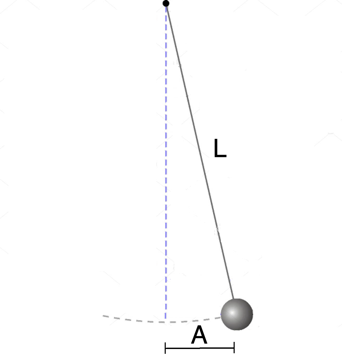
FIGURE \(1.\) Simple Pendulum.
Now, the above case shows how a relationship, a relationship concerning periodic motion which goes even beyond the concrete system of study, generalizing a whole class of phenomena, can be extracted for a specific system out of the many complex systems, sheer chaos, surrounding us, provided a genius like Galileo gets involved. Equally as important is not only the fact that Galileo was able to establish the above relationship for that chosen system, but that he also foresaw the special significance of that particular system, as opposed to any other system that could have attracted his attention, when sitting on the pew in the Pisa Cathedral, looking up at the swaying chandelier. To lend importance to a concrete object of study and have the profundity of discerning its characteristic relationships that would allow predicting the behavior of any similar system under the same conditions, is a special gift which only very talented individuals dealing with science have, in addition to their training. These abilities are even better expressed in geniuses, who can isolate cases of study possessing great generality and depth.
Complex systems defying solution
The example given with the pendulum, is fortuitously characterized by combining both enormous significance for science, on the one hand, and on the other, the allowance to have the relations between its crucial parameters be fully establishable, so that any time the need arises, it can repeatedly and reproducibly be demonstrated. The latter is a crucial characteristic for a finding to be called scientific. Most findings in this book, especially the basic conclusions, also have this categorical, unequivocal character.
However, there are cases of enormous significance but, unfortunately, by their very essence, they are not prone to anything other than, in the best case, fuzzy understanding of whatever may seem as relations therein. Usually, projects concerning history and archaeology, are presented as examples of such inherent uncertainty. Recently, a global issue, such as anthropogenic cause for climate change, is aggressively promoted globally as some sort of science, which it obviously isnt, especially because of the inherent uncertainties contained therein, to say nothing about the lack of possibility to carry out reproducible experiments under controlled conditions, so that the conclusions drawn can be considered scientifically drawn. It is very important not to mislead the public that some activity is scientific, when actually it is obviously notwe cannot turn back time, and again make history, let alone ensure the same initial conditions, to say nothing of carrying them out under controlled conditions, in order to claim scientificity of the historical claims we make. The same applies to archaeology, as well as to medicine. Medicine is not science and presenting it otherwise is very dangerous, especially due to the interest the majority of people have regarding their health. Such misrepresentation may be even deadly.
One can understand why medicine is not science not only by considering that in science conclusions drawn can be absolutely unequivocal, as the conclusion that the theory of relativity is absurdity, or that quantum mechanics must be replaced by classical mechanics, as evident from the arguments provided in this book, but also when considering experiments. Take, for example, Boyles law connecting pressure \(p\) and volume \(v\) of a gas in an enclosed vessel at constant temperature \(T\) (more on notation is given below), yielding \(PV = const\). This law can be demonstrated anywhere, at any time, provided the gas contained in the cylinder has the properties of ideal gas and the conditions of the experiment, determining the state of the system (cylinder and gas), especially temperature, are kept the same. At a constant temperature, any change in volume of the cylinder leads to such change of pressure, which maintains the product of volume and pressure constant. That can be proven with any cylinder and any gas, as long as the gas has the properties of an ideal gasFIGURE \(2\). This is absolutely not possible to be done in medicine, where every individual; that is, the system to be studied, is different and is subject to a myriad of known and unknown parameters affecting ones health.
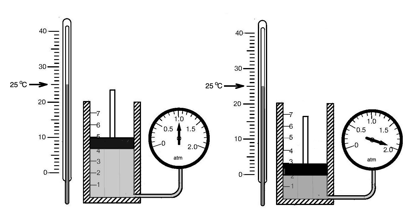
FIGURE \(2.\) Schematic of the apparatus to observe Boyles law. For a given temperature of 25\(^{\circ}\)C (298K). The product of volume of ideal gas and its pressure read from the pressure gauge, is equal to a constant: \(PV = 1 \times 4 = 2 \times 2 = const\).
One should not be confused by the fact that proving both Boyles law and a medicinal claim involves statistics. In the case of Boyles law, the relations involving statistical quantities such as pressure and temperature, can be established exactly through a reproducible experiment carried out under conditions whereby all the parameters are under control.
On the contrary, in what may appear as an experiment in medicine, the statistics which can be applied on a sample of a population can never be scientifically rigorous, so that the results can apply unequivocally to every single individualconversely, think of absolute rigorousness and exactness of Boyles law application to every single cylinder containing ideal gas, used to prove Boyles laws validity.
Recently, interest in vaccines has been created, if the experimental potions injected massively have at all the characteristics of vaccines, let alone abiding by the required minimum criteria for vaccine testing. Speculations presented as truth abound on both sides, pro and con, and on top of the inherently non-scientific character of medicine, the greed and unscrupulousness of the corporate world grips the nations, using governmental power for those corporations profitable but inhuman role. Their powers are too great for one to expect any impact by sanity and honesty, the goods of least interest to the corporate beasts. At least, individuals should know the truth that truth about medical problems is fuzzy. It is individual. Of course, individuals must be conscientious and feel social responsibility but that does not invalidate their individual response to a medical problem, which typically is a complicated matter, not prone to exact science. The procedures applied are shaped in the boxes of schemas and are predetermined, and if it doesnt fit you, thats too bad. Profit-driven medicine, the post-modern, post-industrial world, marketizing every possible human activity, devoting it, on top, only to service economy, the world that has forgotten all of its humanistic streak, caring only about creating services it can sell, couldnt care less about what the individual really needs, as long as that brings profits to the corporations. This is, however, a whole different discussion, interesting and important, discussed in another book of this author, entitled No Great Reset, but now we have work to do. Therefore, let us begin dealing with the topic at hand.
Academic tone
When someone crosses the border of elementary academic decency and integrity, hoping to get away with anything, even lies and deception, shamelessly presenting it as genius science, especially using it to achieve prominence, and thus governance over the scientific thought process, the academic tone becomes out of place.
Otherwise, hypocritically keeping the usual even academic way of expression, would make it appear, not only to the outside world, but also to the collegiate not immediately involved in the question, that everything is OK, that it is a common scientific discourse with its disagreements and divagation, and that foisting conclusions based on the assumption that two unequal things are equal, adopted in order to arrive at the desired formula at any rate, as the author of refs.\(^{2-4}\) has persistently brazenly done as a staple, a signature of his style, is something in the order of things in academic science, worthy of dispassionate discourse, let alone comprises science of the highest order. On the contrary, such objectionable practice is the real violation of academic behavior, even beyond only violating academic tone.
Therefore, abandoning academic tone, within reason, is not only fully justified, but is even needed, in order to emphasize the outrageous nerve someone having the turpitude of calling himself scientist, pronounced even as genius, having the temerity to infest the world with his bland mediocrity.
The polite, good bourgeois manners, are forgotten when an intruder invades a salon-party, crushing furniture and attacking the guests. Police, called to restore order, have no second thoughts on behaving outside the salon manners of the polite ball-party society. Destruction on a wide scale done by insolently faulty science, shoved down the throat of society, is not visible, but it is not less damaging to the intellect, especially of the youth, than the material damage caused by the open display of brute devastation.
The usual impassionate style of academic writing must be broken when such unusual invasion of brazenness takes place. Tolerating it, glazing it over with politeness, makes one a co-conspirator in the travesty, enabler of the highest intellectual crime that might ever occupy the scientific world.
Socially, criticism of established notions, even if these notions are outrightly faulty, is not viewed favorably. More often than not, the one criticized, even if the criticism leveled at him is justified, is perceived as the underdog. The public by and large, as a matter of simple human psychology, roots for the underdog. This furthers the opportunities for the wrong views, once they have found a way to sneak in, to get an even deeper entrenchment. Needless to say, that greatly helps the deceiver in legalizing and promoting his iniquitous actthe perpetrator of deception and absurdity, astoundingly, becomes an untouchable fixture. That is not some imaginary scenario but is a living truth as we speak. As a result, matters have deteriorated to such an extent, that one often hears that the critical analyzer, no matter how correct and honest, is viewed as a villain criticizing the great man with the sole purpose to make a name for himself on the back of an established genius, or to accrue various other social and material benefits by name-dropping. That is too bad, however, because, especially in real science, proof is in the pudding for the uncorrupted student of nature. The proof is laid out widely in front of his eyes, as is done in this book, as well as in the other books and writings of this author. Ignoring this unequivocal proof, shadow-banning it, may occur only due to deeply vested interests and various other underhanded motives.
Terminology and content of some notions used
Without getting into the history of the question, several pivotal moments need to be mentioned, in order to bring more clarity to a question wrapped in a great deal of unjustified mystique.
However, before continuing with quantum mechanics, which is the topic at hand, some notions are mentioned, which I think need an introduction, especially notions that may even cause confusion. Because I am not the reader of the book, it is not unusual for someone to resort to explaining some matters, while at the same time other matters are creeping into the conscience of the reader that require more clarity. I most certainly will miss some notions which are in need of more explanation. In the course of time, however, as the book begins to find its way amongst readers, additions may be made to address issues which at this moment I have failed to see the need to address.
NotationTo save space and to make referencing easier, henceforth the quantities are denoted mostly as it is done in the respective papers. For example,
Denoting absolute temperatureif the discussed paper denotes the absolute temperature by using the Greek letter \(\theta\), so will the absolute temperature be denoted in this book. Usually, the absolute temperature is denoted by the letter \(T\) and that would also be a way of denoting absolute temperature in this book.
Denoting natural logarithmAlso, \(\log\) and \(\ln\) are two equivalent ways to denote natural logarithm (logarithm with a base \(e\)) in this book. The former is the convention in many of the papers discussed herewith, and also this is the convention used by the mathematical facility Wolfram Alpha on the internet, often employed in this book to verify equations and graphs. We will use both symbols depending on the context.
Dashed vs. solid boxA dashed box enclosing a formula is used to make the incorrect formulae stand out and be distinguished from the correct formulae, sometimes enclosed by a solid box.
Frequency\(\nu\) may be thought of as the number of times per second the crest of a wave is passing a given point, while wavelength \(\lambda\) is the spatial distance between two crests or between two troughs. Frequency and wavelength of electromagnetic waves are related as \(\nu = \frac{c}{\lambda}\).
UnitsThe units of the quantities will be given only occasionally, when it is deemed necessary for the understanding of the matter discussed. For easier comprehension the units of quantities will be presented, whenever there is a numerator and denominator, as quotients enclosed by bracketsas \(\left[ \frac{kg \ m}{s^2}\right]\), rather than as \(\left[kg \ m \ s^{-2}\right]\). As another important example, the units of the universal gas constant \(R\) would be given as \(\left[ \frac{J}{K \ mole} \right]\), instead of \(J \ K^{-1} \ mole^{-1}\), as is usual in some scientific publications.
To avoid clutter, in more than a few instances presenting of units of the quantities is implied and is clear from the context.
Speaking of units, unfortunately, it is not uncommon for standard texts to spend too much time on details and numerical examples, flowing fast over the real problems, to the detriment of clear understanding.
Usually, in the exposés on blackbody radiation, attention is drawn to side issues or various insubstantial distracting details, turning the narration into a very complicated read, while ignoring the really dramatic problems which infest the question. These problems are so grave that they may even require abandoning the subject of analysis.
This kind of intentional or unintentional obfuscation concerns, for example, the units with which the blackbody formula expresses energy. The usual expectation is that it would be energy density; that is, energy per unit volume. However, we are bombarded with other more complicated units which may have utility in engineering but, in fact, do obfuscate the physical grounds of the argumentation. In this book we will try to keep things simple and will stick with energy density within a frequency interval \(\nu\), \(\nu +d\nu\). We will observe Plancks formula for the spectral distribution of energy predominantly in the frequency variant of the formula, although, those curious to see how it can be converted into the wavelength variant can visit Curious mathematical detailExpressing the obtained \(u_{\nu}\) as a function of \(\lambda\).
We should also mention that in addition to sparingly devoting time on established basic things, widely found in the standard literature, mentioning them in passing, we try to apply every effort to excuse the authors and find solutions to what appears as discrepancies and even irresolvable problems. Unfortunately, at times, the authors do not help much by avoidance of clearly defining the quantities they use, and this requires some kind of sleuth work to discern the real meaning of these quantities.
\(\textbf{Volume \(\pmb{v}\)}\)One may see an author stating, for example, consider radiation that occupies a volume \(v\). Usually, physical chemistry denotes volume by upper case \(V\), while the symbol \(v\) in lower case, is reserved for denoting specific volume; that is, volume referred to a unit mass or, most conveniently, referred to \(1\) molemolar volume. In the context of blackbody radiation, it would be \(1\) mole of resonators. In such a case, we speak of molar volume of resonators. The notation \(v\) for specific volume may be confused with velocity \(v\). Every effort will be made to separate these two quite different quantities within the context of the discussion. Because we will be talking most of the time about volume \(V\), rather than specific volume \(v\), that makes it even easier to distinguish between the two terms.
Of course, it is another story if we can at all attribute the concept of a molar volume, \(v\), to one mole of resonators in a cavity. If we do, and that attribution we undertake in order to resort to the ideal gas law \(PV = 1 \cdot RT\), written for \(n = 1\) moles of gas, then we, indeed, can write \(v = \frac{1 \cdot RT}{P}\), and then we would be attributing (wrongly, as we will see later) the particle-like properties of the ideal gas to the non-particle-like continuous electromagnetic radiation. C. I. Noninskis view\(^{11}\), derives portions of energy exchanged between the parts of the system such as the oscillators, which are the real physical quanta. However, in C. I Noninskis work the notion of these exchanging heat quanta arrives from legitimate classical principles of physics, not from a thermodynamic system such as the ideal gas law, despite the fact that the ideal gas law is completely legitimate in its own right.
Furthermore, the premature attributing of thermodynamic properties; that is, of particle-like properties, of ideal gas, to electromagnetic waves, plunges the analysis into a logical fallacy. It is exactly the fact that electromagnetic radiation would have ideal gas properties, is what is supposed to be proven, not assumed. In other words, one would be committing petitio principii if one jumps the gun and goes ahead, attributing the properties of an ideal gas to electromagnetic radiation, prior to proving that electromagnetic waves indeed behave as an ideal gas. It is shown in this book that, unfortunately, such logical fallacy has been committed not only with respect to the thermodynamic-electromagnetic analogy, but also with respect to other claims, which, sadly, are forming the flawed structure of contemporary physics.
Further, it is obvious that molar volume \(v\) is equal to the quotient of the molar mass \(M\) and the density \(\rho\): \(\frac{M}{\rho} = \frac{M}{\frac{m}{V}} = \frac{V}{\frac{m}{M}} = \frac{V}{n} = v\), where \(m\) is the mass of the gas and \(n\) is the number of moles. What is really interesting, however, is that Avogadro has discovered that equal volumes of any gas behaving as an ideal gas consist of the same number of particles (we usually use the word molecules, or, more seldomly, atoms, to signify these particles). Therefore, the reverse stands to reasonequal number of particles of ideal gas occupy the same volume at Standard Temperature and Pressure (STP), or if this number of particles is exactly \(1\) mole, then \(1\) mole of any ideal gas must occupy the same volume and that particular volume, occupied by \(1\) mole of any gas, is 22.4L. Thus, if \(v\) indicates the molar volume of a container with \(1\) mole of resonators, and if we agree to commit petitio principii by attributing thermodynamic properties to radiation, then the molar volume \(v\) of this many resonators would be just the same as the number of any ideal gas molecules; namely, 22.4L at STP. It would be prudent, however, not to continue this analogy, prior to observing the reality of situation (just as a heads-upthis analogy fails).
If that similarity is not assumed and attempts are made to prove it, then it will be seen that the \(v\) of the enclosure, even if it contains \(1\) mole of resonators, cannot be considered to be 22.4L at STP. The lack of analogy between the relationships characterizing electromagnetic waves, on the one hand, and on the other, the thermodynamics of an ideal gas, indicates that Avogadros hypothesis does not apply to electromagnetic waves.
Notably, however, when the realistic picture of exchanging energy (heat) between the parts of the system, proposed by C. I. Noninski\({11}\) (cf. facsimile), is adopted, the description of a system of finite entities, quanta, becomes natural, comprehensible, and completely describable by classical physics.
One more thing, it may be noticed that in this book pressure is denoted by capital \(P\). Some texts write it in lower case \(p\). Both are correct, as long as when talking about pressure, writing it as \(p\) does not confuse it with momentum, and when writing it as \(P\), does not confuse it with power. This distinction usually becomes clear from the context.
Oscillators vs. resonatorsAlthough there may a subtle difference, if at all, whereby an oscillator may be looked upon as an active entity, in opposition to the resonator which vibrates under the action of a stimulating external electromagnetic field, in this book we will use these terms interchangeably, in view of the coincidence of the expressions describing the properties of these entities of interest herewith. Planck prefers to use resonators in his studies, while C. I. Noninski uses oscillators.
Displacement of a free bodyIn order to be physically consistent and in harmony with reality, we will consider real displacement, as opposed to the virtual displacement. Virtual displacement is one of the factors causing confusion in mechanics. This is the first thing we will avoid. The parts of this book dealing with thoughts concerning developments in classical physics practically always observe a free body initially at rest at \(x_{\circ} = 0\) and \(v_{\circ} = 0\), which is then acted upon by a constant force.
Thus,
for brevity, we will consider
1)
The real displacement \(\Delta x = x_2 - x_1\) to have occurred from
\(x_1 = 0\) to \(x_2 = x\) (as opposed to the virtual displacement
\(\delta x\) which is confusingly used in mechanics, and which is
practically not a displacement at all). Therefore, \(\Delta x = x_2 -
x_1 = x - 0 = x\).
2)
The velocity at \(x_1 = 0\) is \(v_1 = 0\), while the velocity at
\(x_2 = x\) is \(v_2 = v\). Therefore, \(\Delta v = v_2 - v_1 = v - 0
= v\).
And,
finally
3)
The time at \(x_1 = 0\) is \(t_1 = 0\) while the time at \(x_2 = x\)
is \(t_2 = t\). Therefore, \(\Delta t = t_2 - t_1 = t - 0 = t\).
When using this symbolism, we are indicating that we are interested only in changes in these values. Therefore, it is immaterial what their beginning values are, taking those beginning values always to be zero.
In some parts of the text, these intervals will be denoted alternatively by \(\Delta x\), \(\Delta t\) and \(\Delta v\), which, although slightly clumsier as notation, would contribute at times to the clarity of exposition, it seems.
Note that by these same symbols \(\Delta x\), \(\Delta t\) and \(\Delta v\) we will also denote uncertainties in measuring the respective quantities.
Operative and non-operative motionAristotle thought that all motion is operative; that is, simply stating, that all motion can be felt. It was Galileo who first discovered that there is a special type of motion, which cannot be felt; that is, which preserves the laws of physics. This is the so-called uniform linear (translatory) motion; that is, a motion at constant velocity \(v\), which is no motion at all. Indeed, it contains in its name the word motion, but, in actuality, it is the same as rest. Thus, for someone who resides in a coordinate system, moving at constant velocity \(v\); that is, lacking acceleration, this kind of motion is undetectable. It is non-operational. Uniform translatory motion is non-operational. This is Galileos famous principle of relativity. Newtons first law has it at its basis. The principle of relativity was borrowed without reference to Galileo by the author of the so-called theory of relativity, only to promptly violate it in his theory. This important principle will be talked about again later in this book, especially regarding its catastrophic violation, rendering the so-called theory of relativity an absurdity.
Exchange energyHenceforth, the terms exchange energy and exchanging energy will be used alternatively to mean heat.
What is a function?Perhaps, it would be useful to refresh memory by recalling what is to be understood under the term function or functional dependence. For the purposes of this book, the first thing is to realize that there is a quantity called the independent variable, usually denoted by \(x\), many times by \(t\), or by any other letter. The independent variable is free to acquire any value, usually acquiring successive values. Of course, this is not much to say. So what, that we can have randomly chosen values of a quantity? Nothing much, if that were the only thing to say and do. The big deal, however, is that we have to realize having at hand such an entity, which happens to enjoy the freedom of acquiring chosen values, in order to be able to impose on that value restrictions, which transform it and lock it into another value. These restrictions, this rule, fixing the independent variable in a particular alternative way, is the function. This is the mathematical shell which ensures what exact mapping must be imposed on the value of the independent variable, so that the independent variable be turned into a particular fixed different value. So, one uses the independent value \(x\) in question, to have it plugged into some mathematical formula, in order to calculate a value. For instance, we have at our disposal the independent variable \(x\). The concrete function, the shell, of interest may be, say, the square root; namely, \(\sqrt{ \ \ \ }\). This shell, this instruction, \(\sqrt{ \ \ \ }\), tells us that every \(x\) we may think of should provide as a response \(y\) not just any \(y\), but exactly the response equal to \(y = \sqrt{x}\), and nothing else in this case. As a result, we say \(y\) is a function of \(x\), and we are lucky to know exactly what function of \(x\) that function \(y\) iswell, in this case it is nothing other than \(y = \sqrt{x}\). This book is strewn with functions, and each function consists of its own shell or, call it, rule, which is determined by the physical situation that function is supposed to describe.
What is the state of the system?The state of a system is characterized by a set of parameters, enough to determine all the properties of the system.
What is a process?Induced or spontaneous change of the defining parameters of the state of a system, changing the state of the system, constitutes a process.
What is statistical distribution?There are terms such as Gaussian distribution or Poisson distribution encountered in this book. Even Plancks or Wiens blackbody formulae are referred to as distributions. What does that mean? Statistical distribution provides the assembly of sequential outcomes, referring to a set of conditions. For example, there is a certain intensity of emission, which corresponds to every value of the wavelength \(\lambda\). The assembly, put together, usually in a graphical form, represents the distribution of these intensities along, say, increasing value of \(\lambda\). This distribution may also be expressed in analytical form, as a function, whereby to every wavelength \(\lambda\), there will be a corresponding value of intensity, shaped by the kind of function we use. Since one may encounter the term normal distribution (Gaussian distribution) or normal spectrum, the simplest definition that can be given to this detail for our purposes, is that these terms refer to the approximate model of sequentially plotted wavelengths (frequencies) and their corresponding intensities (energy densities).
Obviously, the kind of function we use had better be correct, so that the value which comes out as a result of the functions crunching, coincides with the experimentally observed value for that \(\lambda\). Some functions, proposed for such description, do not follow the experimentally found distribution. Such is the function proposed by Rayleigh and Jeans. The best function proposed for the purpose is provided by Planck. It fits the experimental curve perfectly. Unfortunately, Planck was not able to derive it, as will be shown. The fact that in the end he came up with the correct form of the distribution function does not prove that he has derived that function correctly (he has not), because obtaining the correct mathematical expression alone can be done any time by using the methods of applied mathematics. This, however, does not amount to deriving the formula on physical premises.
To derive a formula, such as this one, means to base the derivation on certain views describing how nature works under these particular circumstances, and then justify every follow-up conclusion by logically following these foundational views. This, Planck hasnt been able to accomplish. The correct derivation of the blackbody radiation formula was accomplished by C. I. Noninski by following classical views about exchanging energy between the oscillators participating in the system. The fact that following these views leads to the correct formula, is a proof that the views the derivation is based on, are correct, not vice versaas said, coming up with a correct formula, fitting an experimental curve, may be done by applying mathematical methods, which does not prove the veracity of a frivolous initial idea.
Classical physicsIn this book, classical physics or, more narrowly, classical mechanics, signifies physics or mechanics, devoid of any trace of theory of relativity and of quantum mechanics.
On not discussing experimental resultsThis book withholds discussing experimental details. Prior to experiment, there must be a solid theoretical foundation to justify spending such efforts. Quantum mechanics lacks such fundamentals, even less has it solid fundamentals. Furthermore, travesty such as the one presented in ref.\(^{3}\) invalidates itself on the very pages of the paper where it is put forth. It is absurdity. Absurdity can never be contemplated as anything worthy of contemplation, let alone subjecting it to experimental verification. The absurdity is false a priori, and can be the subject of no discourse whatsoever, let alone experimental tests. Similar is the situation with ref.\(^{2}\) and ref.\(^{4}\), whereby there is also nothing to be experimented onthe formulae proposed for experimental verification have not been derived but are a result of deceptive juggling with incorrect premises.
Otherwise, the views of C. I. Noninski, concluding that classical physics derives interaction amongst systems or their parts via discrete portions of energy, rather than as a continuous stream, fit snugly not only with the explanation of photoelectric effect, but with everything else that seemed strange and unexplained, such as the experiments of Davisson and Germer or the Compton effect, to name a few that have befuddled physicists, taken on the wrong path of denial that classical physics may explain those phenomena. Although something will be said in the last part of this book, indicating the direction in which physics ought to develop, a direction having an exclusively classical character, a more thorough observation as to how the mentioned effects and phenomena can be explained classically will be deferred to future writings. This book satisfies itself with laying the theoretical foundations of correct thinking about these phenomena, at the same time requiring radical parting with an incredible intellectual menace that has been infesting physics for over a century, on top of it, having far and wide reaching damaging social repercussions and consequences.
Numerical value of constantsSince the most important thing, because it is exactly what is confusing everyone, is to understand the principle of what is wrong with quantum mechanics and why it should be abandoned, the numerical values of the constants, with some exceptions, will be generally avoided, as will solving of numerical problems and anything else having applied, engineering hue.
Citation of contributorsThis book gives credit only to persons who have real contributions to science. Others are ignored and are not mentioned by name.
How the quantum mechanics madness began
In effect, it all started with Plancks 1901 paper\(^{1}\) trying to explain the experimental results connected with the emission of the so-called blackbody, a paper to be discussed shortly. There were some earlier efforts of his, as well as studies by him on the topic after 1901. However, the 1901 paper really presents in sufficient detail what are claimed to be the founding ideas of quantum mechanics, as far as its physical background goes, and therefore, we will limit ourselves to observing that particular paper, showing its really flawed nature, without any other introduction to the so-much celebrated, albeit misunderstood, quantum idea. Furthermore, as will be seen, the idea of quanta, in its true sense, is inherent in an area of physics, none other than classical mechanics.
What is a blackbody and why is it so important in physics?
The mere mentioning of blackbody and its radiation often invokes spooky thoughts and an eerie interest in something, which is of much more prosaic nature than the uninitiated public imagination endows it with. It is quite probable that the unusualness of the idea and even the naming itself of the subject of study, was one of the vehicles that helped the subject to capture the public fascination.
It may be something, on a purely psychological level, to the out-of-the-ordinary appeal when hearing the word blackbody, because the blackbody, even as it is an object of study in physics, is indeed a peculiar physical object which, when in equilibrium, is, ideally, capable of 100% absorption of all frequencies of the incident radiation, as well as emitting 100% of all frequencies of the absorbed radiation. Not all objects have such a propertymost objects, in addition to absorbing, are also reflecting part of the incident radiation.
This property of full absorption-emission compensation of radiation at equilibrium, is crucial to understand for the derivations to follow. One important reason to comprehend the above absorption-emission symmetry, is its use by Planck in his treatment of the resonator, placed in an external radiation field.
As a model for his theory, Planck uses what he calls an irradiated, monochromatic, vibrating resonator. This is an oscillator capable of vibrating at the same frequency \(\nu\) as the frequency \(\nu\) of the external field in which that resonator is placed.
Unfortunately, Plancks treatment collapses too soon, as will be seen shortly, driving that otherwise useful model into a dead-end. The full use of that model was accomplished by C. I. Noninski, who was able to derive the law of blackbody radiation, basing his derivation on purely classical principles.
The blackbody, being a very special kind of an object of study, which, as pointed out, unlike other objects, is capable of absorbing 100% of the incident radiation and, reciprocally, is capable of 100% emission of what has been absorbed, allows for the following trick Planck uses in his derivation. Thus, he cleverly sets himself to study not the emission, which he does not have access to, but what, as the condition of the problem, the blackbody receives as an absorber.
That amount, available to the blackbody to absorb, is equivalent to what the blackbody would emit. Exactly this property is used by Planck to draw conclusions about emission, when he, in fact, is studying absorption; that is, stimulating, transferring energy to a resonator by an electromagnetic field of a given frequency.
Therefore, by imparting via a stationary field of energy to the resonator at equilibrium, that acquired energy serves to represent also the emitted energy, of interest to the student of blackbody radiation. The just said explains away the worries of some as to where the emission part in the name of the law comes from, since Planck considers resonators placed in an external electromagnetic field, which is the external provider of energy. Nevertheless, it is the reciprocal absorption-emission property; namely, the blackbody not only absorbing all frequencies but also emitting all frequencies, what resides at the bottom of Plancks derivation.
As said, unfortunately, the use for Plancks model ends here.
The model of a blackbodycavity and resonators
Now, because Plancks work is not the end of the blackbody study, especially because it is flawed, it is important to understand, as a first step, what can be a model for a blackbody. Is it just an imaginary object, or can it be manufactured as a physical contraption, ready to be used for experiments in the laboratory?
The usual model of a blackbody serving as the emitter of the studied radiation is, after all is said and done, the small hole in a hollow enclosure, FIGURE 3.
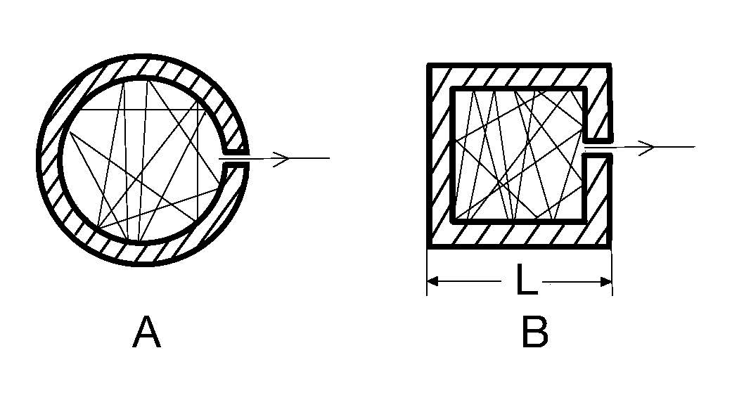
FIGURE \(3.\) Blackbody cavity: Aspherical model; Bcubic model used in the present discussion.
The enclosure has its internal walls covered with soot. Upon heating and then maintaining at a constant high temperature, the hole begins radiating visibly, that visible emission being part of a continuous spectrum of all frequenciesat lower temperatures the blackbody will also radiate but the pinhole appears dark to the human eye because the maximum of emission is out of range from the frequencies the human eye can see. Special infrared (IR) cameras are needed to register the radiation. What is quite interesting to note is that, contrary to expectation, the intensity of emission (radiation) at a given temperature differs for the different frequencies (cf. FIGURE 9). This distribution of intensities over frequencies, respectively, over the wavelengths, is exactly the matter of experimental study and follow-up explanation, the most adequate of which is being unduly credited by the mainstream to Planck.
The fact that the mentioned pinhole, representing a blackbody, emits radiation at all wavelengths, is a very significant property, because many emitters which are not blackbody emitters, do so only at given wavelengths, which, on the other hand, is a lucky circumstance when these emitters are used in the methods of analysisthe presence of certain unique spectral lines proves the presence of a certain element for which these particular lines are characteristic. Obviously, for the lack of radiation at certain wavelengths, they are unsuitable for the studies undertaken to understand the blackbody radiation distribution. Similar are the absorption spectra, whereby an object is capable of absorbing only certain wavelengths.
On the contrary, the blackbody has no such problems. It emits at all wavelengths, \(\lambda\), and therefore is a perfect source for the study of the distribution of intensities of radiation with wavelength, respectively, frequency.
The instrument to study blackbody radiation
For the purposes of such study; namely, studying the intensity at each wavelength (respectively, frequency), a slit is placed in front of the emitting pinhole of the blackbody enclosure, then the narrow beam formed is passed through a prism secured on a rotating turret, FIGURE 4.
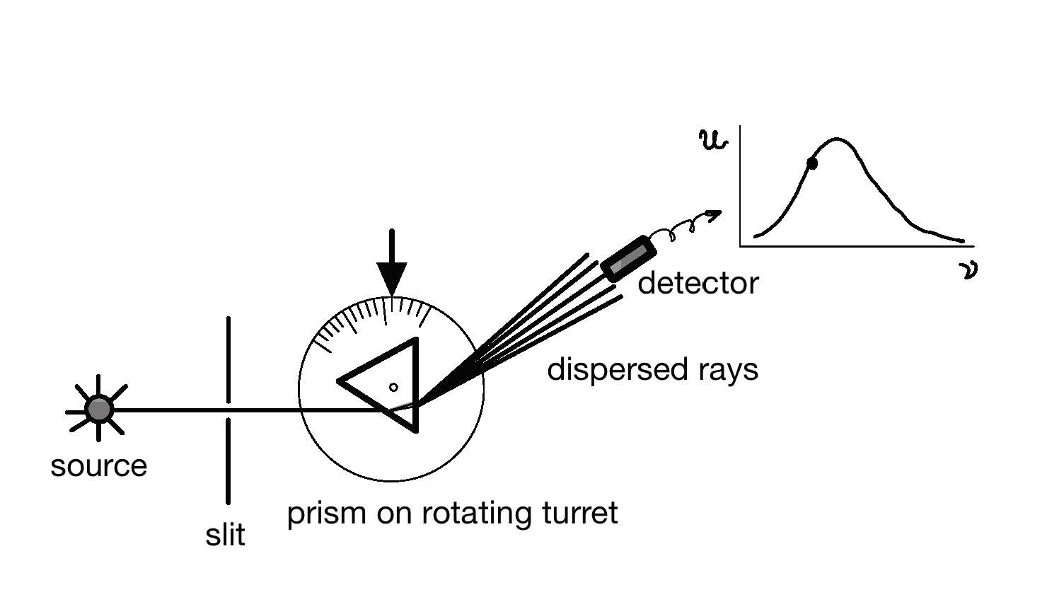
FIGURE \(4.\) Schematic of the apparatus for the study of blackbody radiation.
The prism resolves the beam into a continuous fan of rays of different frequencies (colors), further directed (collimated) sequentially, by turning the turret, onto a detector called a bolometer, measuring the change of resistance due to the increase of temperature caused by incident electromagnetic rays. Other, more modern sensors of incident electromagnetic rays, sensitive to all wavelengths, may also be used.
The detector converts the incident radiation into an electric signal of magnitude which depends on the intensity of the falling ray of a given wavelength (frequency). Modern instruments use multi-spectral detectors, while as a source of blackbody radiation, even the glowing Tungsten filament of a common bulb is used. As a matter of fact, lecturers often entertain their students by pointing out that the Sun can also be considered a blackbodya seeming paradox. There is no perfect blackbody in nature and the closest to a blackbody is the mentioned hollow cavity (enclosure, contraption, void) with a pinhole, cf. FIGURE 3). At every temperature, the inside soot-covered walls of the cavity emit and absorb radiation, which reaches equilibrium, and is not affected from the outside because the small size of the pinhole, allowing only a tiny amount to get out, used for testing, is too insignificant to affect what takes place in the cavity, thus, not disturbing the equilibrium established inside. Nevertheless, when the temperature is raised, the hole begins to emit radiation even in the visible spectrum, as was already said.
Here is something most interesting. It turns out that if the enclosures are made of different materials, consequently their outer bodies, although kept at the same temperature, displaying different colors upon bringing them to that temperature, the color of the pinhole stays the same for the enclosures made of different materialsthe blackbody radiation is independent of the material of the enclosure. It depends only on temperature.
The light of each wavelength falling on the detector, invokes a different current representing intensity. The intensity corresponding to the different wavelengths, represented by the current generated in the detector, is plotted against the wavelength \(\lambda\) and what is observed is something quite peculiar. The graph of these intensities as a function of wavelength \(\lambda\) goes through a maximum, which shifts to the lower \(\lambda\) values (shorter wavelengths) as the temperature rises (cf. FIGURE 11). In general, even not considering blackbody radiation, when a piece of metal is heated, with the increase of temperature, from a certain temperature on, the metal piece begins glowing.
In passing we will note that this phenomenon of shifting with the increase of temperature, of the emission maximum to the left, to the lower \(\lambda\) values, described by \(T \lambda_{max} = const\), was discovered by Wien and is known as Wiens displacement lawsee the ADDENDUM. In the same paper, Wien has also derived his distribution law; that is, a law describing how intensities of blackbody radiation change with wavelength (respectively frequency), a law very close to the law, correctly derived by C. I. Noninski. When talking about Wien in this book, we will always have in mind his distribution law, not Wiens displacement law.
Absolute truths as basis of inquiry
Before going further in our journey, we must make it perfectly clear that science is about truthnot consensus amongst various expertsbut truth. The more an intellectual pursuit depends on consensus, the more it deviates from qualifying as science. Reaching truth is a difficult endeavor. Nevertheless, truth is the goal, despite the seemingness that an agreement amongst experts may be a substitute for truth. Many times, agreement amongst experts is the most we can achieve, adopting it as relative truth, considering the difficulty of the problem, but that must not give us the feeling that such agreement is enough and we may rest on our laurels as scientific achievers. On the contrary, we must pursue, even if we remain alone in the world, the objective truth, which in many instances may turn into the final, absolute, truth regarding the studying object and its properties. Moreover, that there are glaring instances when the whole world has achieved consensus and there is not a single soul, let alone an active scientist, who would disagree with the collectively adopted doctrine, yet every single one may unequivocally convince himself in its wrongness, should he really care about the truth. Incidentally, in the nineteen sixties, the term paradigm was invented to signify that collective adoption of a doctrine, the emphasis being on collective, not on whether or not that doctrine is correct. Thus, the individuals in what may be considered a scientific setting are required to abide by the collectively accepted doctrine, the paradigm, no matter if it is a deception, absurdity or an outright lie. If the collective holds it as a paradigm, it becomes a law for all its members. Those who dissent soon find themselves out in the cold.
Thus, if one decides against all odds to be true to sciencethe uncompromising protector of truthturning his back on the paradigm, one has no choice but to acknowledge that there is one single, unequivocal, truth about a physical phenomenon.
In particular, there is one and only one unequivocal truth about the mentioned theory of relativity, and it is that the theory of relativity is an absurdity, and therefore it must at once excuse itself from physics. That the theory of relativity is an absurdity is an absolute truth. The shining example of the establishing the absolute truth about the theory of relativity must be our guiding light in all our endeavors in science. Efforts to personally look for the absolute truth about a question of interest, and personally confirm its veracity, must be established as the most desired principle in scientific research. That principle will be applied to the discussions and conclusions in this book.
Thus, in our quest for truth with respect to quantum mechanics, we will strive to base our inferences on deductive reasoning as much as we possibly can, the way it was possible when analyzing the theory of relativity.
Thus,
in principle, when facing questions which seem insurmountable, the
safe shore to start from is to begin
\(\boxed{pondering \ \ the \ \ inevitable \ \ absolute \ \ truths \ \
of \ \ physics}\)
connected with the question. This will be our guiding light when facing a difficult question causing us to wonderwhere do I start?
This book provides ample examples of such a way of tackling matters which otherwise, starting in the middle of things, without clear, unquestionable definition of what is being sought and where to start from, may be a point of confusion for life.
Following this method of beginning with what is firmly established, and delving into the abyss of the unknown, will untangle the seemingly muddled subject of quantum mechanics, as well as any other complex topic, and will make it easy and enjoyable, because of the satisfaction brought by bettering the understanding of the matter, despite the disappointment that such enhanced understanding would make it imminent to leave behind the topic that is said to hold so many promises.
The necessity of the search for absolute truths
Probably at all times, but especially in todays world, overwhelmed as never before in history by various means of prompt world communications, what can be believed has become an ever scarcer rarity. So, there should be some way for the individual to separate the wheat from the chaff. This has become vital for the very existence of the world societies. The problem is aggravated even more by the inevitable difficulty of determining who the judge would be. Therefore, anything said should be juxtaposed to self-evident, self-explanatory statements, whose veracity no person of average intelligence could deny. This is what this book defines as absolute truths.
Definitions of physics as absolute truths
It should be clear to anyone of average intelligence that the definition of velocity referred to a body in a given system of reference, is fixed. The definition of velocity is an absolute truth. Velocity, \(v\), is always distance, \(s\), over time, \(t\), even if these are expressed in infinitesimal terms; i. e., as \(\frac{ds}{dt}\), \begin{equation}\label{velocity} v = \frac{s}{t}. \end{equation}
This definition has purely physical meaning and is not restricted mathematically. Mathematics allows any number to be divided by any other non-zero number. For instance, it is perfectly acceptable mathematically to divide \(s\) by the seventh power of \(t\) \begin{equation}\label{novelocity} \frac{s}{t^7}. \end{equation}
Eq.(\ref{novelocity}), however, does not express the physical quantity known as velocity. Eq.(\ref{novelocity}) has no physical meaning if one intends to use it as the definition of velocity, although mathematically eq.(\ref{novelocity}) is fully acceptable.
The above example should help those who elevate mathematics to the be-all and end-all in physics, understand that not all mathematical expressions, even though correct, have physical meaning.
Thus, even if someone postulates that \(\frac{s}{t^7}\) should be considered velocity, such postulate will be unacceptable from the physical point of view, and no conclusions based on such postulate will have any place in physics.
Furthermore, senselessness in physics is detected even when something truthful is presented as a postulate and then it is misinterpreted. A prominent example in physics of such sort of senselessness is the second postulate (the velocity of light constancy) in the theory of relativity. Emphatically, it is absolutely not necessary to discuss the second postulate in any context because the theory of relativity falters as early as the disastrous application of the otherwise correct first postulate (the principle of relativity discovered by Galileo), a faltering which is enough to altogether overthrow said theory of relativity. This unequivocal proof of relativitys absurdity has its place in this book as well, as an illustration of the general failure to employ correct thinking.
However, despite the absolute waste of time which discussing what is foisted as second postulate of the theory of relativity would be if one decides to do it, we will now say some words just for entertainment and fun.
The fact that light emitted from a light source at rest with a coordinate system has homogeneously (in all possible directions) a constant velocity c was established experimentally by Michelson and Morley \(^{18}\). Once this physical law has been established, then there is nothing knew to know, let alone pronounce it as a postulate (the second postulate of the theory of relativity), that when in one system of coordinates the light emitted from a light source at rest with that system has homogeneously constant velocity, then the light emitted from a light source at rest with another system, in uniform translatory motion, will also have homogeneously constant velocity. This is exactly what the principle of relativity, which the author of ref.\(^{3}\) has borrowed, without even referencing the discoverer of that principle, Galileo, mandates.
Again, this is no postulate at all but is a physical fact, a law, found experimentally prior to even a thought about the theory of relativity. Furthering of this discovery, by adding that ref.\(^{3}\) also implies constancy of light velocity for a source of light which is moving in a system of coordinates, portraying that this property of light is also included in what has been pronounced as the second postulate, is obviously wrong, because that is exactly what Michelson and Morley disproved.
The claim that a light source, moving in a system of coordinates, would give rise to light having constant velocity c, without adding (or subtracting) the velocity of the source itself, would have been true if, after the emission, the velocity of light would have become the property of the undulations of an imaginary figment, known as ether. With their null result from the experiment, Michelson and Morley proved unequivocally the non-existence of ether. Thus, if anyone imagines constancy of light velocity, independent of the light source velocity, he must consult the experiment of Michelson and Morley, which was the first experimental proof for the invalidity of such fantasy and if one imagines that this kind of light constancy constitutes the fundamental feature of the theory of relativity, the outcome from Michelson and Morleys experiment would be enough to convince him otherwise. Curiously, there are still people and laboratories proposing to the Government to fund them for experiments to establish the veracity of what they perceive as a second postulate. They should know that they need not apply for grants for something that has already been establishedMichelson and Morley have already established experimentally that no such twisting of their finding is at all possible. Not adding (or subtracting) to the velocity of light the velocity of the source, goes against the laws of nature.
The wrongness of understanding of Michelson and Morley result, wrongly pronouncing it as a postulatethe second postulatethat confused understanding, as well as many other problems infesting the theory of relativity, arise over and above the catastrophic failure of the theory of relativity, invalidating itself on the very pages of its founding 1905 paper by violating the principle of relativity (its first postulate), and one can only spend time on these infestations, treating them as unfortunate curiosities, once that catastrophic violation of the first postulate gets across to him.
The understanding that the definition of velocity and acceleration are absolute truths in physics, will immediately lead us to deriving another absolute truth, which will determine that our understanding of motion must change. That absolute truth, which we will deal with shortly, is the inevitable change of velocity when motion takes place. This inevitable velocity change we will elevate to a fundamental principle in mechanics, and the equation it follows from, as the basic formula of mechanics.
For some reason, most profound consequences arrived at from nothing other than absolute truths, have not been paid attention to, and that dealing with that omission is obviously long overdue, considering the shambles physics is in today, resulting from such an inauspicious looking omission.
It was shown in a number of papers, such as ref.\(^{19,20}\), that under certain conditions, the conservation aspect\(^{60}\) of the principle of conservation of energy (CoE) can be violated through ensuring opportunities, provided by the specific construction of the machine, for motion to be induced spontaneously by conservative forces (gravitational, magnetic etc.) Spontaneous inducing of displacement under the action of these conservative forces is nothing other than spontaneous obtainment of energy without extracting it from a pre-existing energy reservoir (so-called production of energy from nothing used as an euphemism\(^{61}\) for brevity of expressing the violation in question). This will be the subject of a future study.
In view of the above, and in principle, the question of the nature of motion is of primary importance. Especially if it can be treated classically. Furthermore, it would be of even greater interest if such classical treatment of motion can be used to explain some of the ostensible puzzles of modern physics, such as the uncertainty principle in quantum mechanics, or the connection between mass and energy, which has already been shown to be not derivable by relativity\(^{21-23}\), demonstrating unequivocally relativitys absurdity, making it the least capable of deriving anything, let alone \(E = mc^2\), as seen here and here. Actually, the first steps to this effect have been made herewiththe part of this book, beginning here, shows that the mysterious phenomena of quantum mechanics are in fact contained in classical physics, provided the concept of motion is correctly understood.
The principle of inevitable velocity change stemming from the fundamental equation of mechanics \(v^2 = 2ax\)
In preparation for what will be discussed in the above-mentioned last section of this book, beginning here, it makes sense to mention, even at these early stages, a principle, first defined by this author, which plays a pivotal role in pointing out the productive directions of classical mechanics development, which charters the road, replacing the dead-end to which quantum mechanics has brought science.
The derivation below of the equation \(v^2 = 2ax\), pronounced in this book as the most fundamental equation of mechanics, reveals that it is another expression of an absolute truth. That most fundamental equation of mechanics determines the principle of inevitable velocity change during real spatial displacement (along the x-axis) of a free body acted upon by a constant force \(F\), or, for short, the principle of inevitable velocity change. Because the free body under investigation is acted upon by a constant force \(F\), it finds itself with velocity uniformly increasing with time; that is, uniformly accelerated with acceleration \(a = const\). This is an important fact, which we will use later. However, what is more important now is the definition of acceleration, which (omitting for brevity the subscript \(x\)), is \begin{equation} \label{} a = \frac{dv}{dt}. \end{equation}
Thus, we can express \(dt\) as \begin{equation} \label{first} dt = \frac {dv} {a}. \end{equation}
On the other hand, from the definition of velocity \begin{equation} v = \frac{dx}{dt}, \end{equation}
we get for this same \(dt\) \begin{equation} \label{second} dt = \frac {dx} {v}. \end{equation}
From eq.(\ref{first}) and eq.(\ref{second}) we have \begin{equation*} \label{} \frac {dx} {v} = \frac {dv} {a} \end{equation*} \begin{equation*} \label{} vdv = adx \end{equation*} \begin{equation*} \label{} \frac{1}{2}dv^2 = adx \end{equation*} \begin{equation*} \label{} \int\limits_0^v dv^2 = 2a \int\limits_0^x dx \end{equation*} \begin{equation*} \label{} v^2\Big|_0^v = 2a x\Big|_0^x \end{equation*} \begin{equation*}\label{expressionforx} x = \frac {v^2} {2a} \end{equation*} \begin{equation}\label{basiclawofmechanics} v^2 = 2ax. \end{equation}
Now, to simplify matters, let the constant acceleration be \(a = \frac{1}{2} \left[ \frac{m}{s^2} \right]\), getting \begin{equation} \label{x as a function of v} v = \sqrt{x}. \end{equation}
Because of the pivotal importance of the derived \(v^2 = 2ax\), respectively, \(v = \sqrt{x}\), we would express here with formulae what was just said above, to avoid even the slightest doubt, that what was obtained, is an expression of velocity as a function of displacement; namely, \(v = f(x)\) from the expression for \(v = \phi(t)\). The expression \(v = \phi(t)\) is a linear function of \(t\), resulting in constant acceleration; that is, \( \frac{d\phi(t)}{dt} = a = const\). In other words, we obtained the parabola expressing \(v\) as a function of \(x\) from the linear dependence of this same \(v\), but as a function of \(t\). Little remarks of the obvious, such as the last one, may be useful sometimes even for someone savvy, because we are all human and may get distracted occasionally. Therefore, the reader may be asked for an excuse for diverting attention to trifles, such as pointing out that the function sought depends on \(x\), not as one always superficially expecting it to be, a function depending on \(t\), standardly having \(v = \phi(t)\) as given.
Also, one needs to be perfectly clear with the physical situation, amounting to the continuous impact of a constant force on a free body which initially is at rest. That is the condition of the problem. Thus, by application of the constant force, the free body is driven out of its state of rest, finding itself, as was said above, with linearly increasing velocity over time, which, when it comes to velocity over distance, is described by the relationship \(v = \sqrt{x}\) upon adopting that the value of \(a\) is \( \frac{1}{2}\) (for brevity, in many instances units will be omitted). In other words, we have an expression which tells us how the ever increasing velocity \(v\) intervals change with respect to \(v = 0\), as the intervals of \(x\) continuously change with respect to their initial value \(x = 0\). Thus, we write \(v\) and \(x\), but these quantities are actually intervals, a notation which was adopted. Of course, that should not be a problem, because the origin of both quantities is the same; namely, zero and what we study is the relationship between their advancing. So, there can be no controversy in this respect with regard to \(v = \sqrt{x}\). It is a completely legitimate absolute equation (coming from absolute truths of physics in the form of two of its definitionsthe definition of velocity and the definition of acceleration).
Average energy of a resonator
Here we will present, as part of the things in physics that cannot be disputed, the standard derivation of the expression for the average energy of a resonator. This known derivation will come in handy when presenting the derivation by C. I. Noninski of the expression for the spectral density of blackbody radiation, based on correct physical premises.
No matter what, particles of a system exchange energy among themselves, and there will always be a constant value of the mean exchanging energy (heat) \(\overline{|\Delta \varepsilon|} = \overline{\Rule{0em}{0em}{0em}\smash{\mathscr{q}}} \), directly connected to the mean energy \(\overline{\varepsilon}\) of the oscillator (resonator) itself. More on this important quantity \(\overline{|\Delta \varepsilon|} = \overline{\Rule{0em}{0em}{0em}\smash{\mathscr{q}}} \) and its direct connection with \(\overline{\varepsilon}\) is discussed here
If we observe a simple harmonic linear oscillator, described by the formula \(x(t)=Acos(2 \pi \nu t)\), the energy \(\varepsilon\) of an individual oscillator, aside from being different for the different frequencies \(\nu\), but, even for oscillators having a given frequency \(\nu\) may also be different due to having different amplitude of vibration \(A\). In this treatment, we will be interested in the average value \(\overline{\varepsilon}\) of oscillators at a given frequency \(\nu\), which obviously infers that all the other quantities in the final formula for \(\overline{\varepsilon}\) will be average quantities corresponding to that frequency \(\nu\). To indicate that an average quantity is had in mind, literature usually uses a bar, \(\overline{symbol}\), above the symbol or angular brackets, \(<\text{symbol}>\), around the symbol. In this book, when it comes to the simple harmonic oscillator, we will use a bar over the symbol only when we denote average energy \(\overline{\varepsilon}\) of the oscillator (resonator).
To derive the expression for the average energy \(\overline{\varepsilon}\) of the oscillator, we will begin with the following fairly obvious equality, in which, by tradition in most standard texts, kinetic energy is denoted by the letter \(T\), while potential energy is denoted by the letter \(V\) \begin{equation}\label{generalmeanenergy} \overline{\varepsilon} = T + V. \end{equation}
Because this is just about the only place in this book (except when using it in the section about Hamiltons equations here and when discussing classical action), where we will see kinetic energy also denoted by \(T\), merely mentioning that here \(T\) does not mean absolute temperature, but our denoting it here as kinetic energy is in keeping with tradition, would be enough. The above general eq.(\ref{generalmeanenergy}) can be easily filled with self-explanatory content. Thus, \begin{equation}\label{unfinishedenergyequation} \overline{\varepsilon} = \frac{1}{2}m \left( \frac{dx}{dt} \right)^2 + V. \end{equation}
Now, concerning explicitly expressing the potential energy \(V\), in this case, instead of using directly Hookes law \(\frac{1}{2}\mathbb{k}x^2\) (notice the peculiar font we use for the spring constant \(\mathbb{k}\), to distinguish it from Boltzmanns constant \(k\)), substituted in the general equation \(E = ax^2 + bv^2\), expressing the fact that the simple harmonic oscillator has two degrees of freedom since its energy expression contains two quadratic terms, to make it a bit more general we will first derive the potential energy \(V\) through expressing the force \(F\) in a general way through potential; namely, \begin{equation*} F(x) = -\frac{dV}{dx}, \end{equation*} solving it for \(V\) \begin{equation*} V = -\int Fdx, \end{equation*}
and only now, considering that in the special case of the simple harmonic oscillator, the force \(F\) is expressed by Hookes law, \(F = - \mathbb{k}x\), we get \begin{equation} V = \mathbb{k}\int xdx. \end{equation}
After carrying out the integration, we obtain for the potential energy \(V\) of the simple harmonic oscillator, derived from Hookes law, the following \begin{equation}\label{oscillatorpotentialenergy} V = \frac{1}{2}\mathbb{k}x^2 + C. \end{equation}
Finally, substituting the obtained expression \(V = \frac{1}{2}\mathbb{k}x^2 + C\), eq.(\ref{oscillatorpotentialenergy}), of the potential energy (considering also that the indefinite integral above turns into a definite integral, causing the constant \(C\) to vanish because of the finite extension of the oscillator from \(0\) to \(x\)), into the equation \(\overline{\varepsilon} = \frac{1}{2}m \left( \frac{dx}{dt} \right)^2 + V\), eq.(\ref{unfinishedenergyequation}), we arrive at the same general equation \(E = ax^2 + bv^2\), containing two quadratic terms (which, as known, amounts to two degrees of freedom, because the \(E\) depends on two independent quadratic terms), presented in a concrete, more detailed form \begin{equation}\label{moredetailedoscillatorenergyequation} \overline{\varepsilon} = \frac{1}{2}m \left( \frac{dx}{dt} \right)^2 + \frac{1}{2}\mathbb{k}x^2. \end{equation}
However, now, we will go further even than eq.(\ref{moredetailedoscillatorenergyequation}), by substituting the equations which define the linear harmonic oscillator. These are trivial substitutions, as well as a derivation that exists in the standard literature, but their immediate availability here may be useful in the context of this book. Thus, if we observe a simple harmonic oscillator, described by \(x(t) = A cos(2 \pi \nu t)\) (which will be used below also in the form \(x =A cos(\omega t)\)), where \(A\) is the amplitude, and substitute that expression for \(x\) in the above eq.(\ref{moredetailedoscillatorenergyequation}), we obtain \begin{equation} \overline{\varepsilon} = \frac{1}{2}m \left( \frac{d(A cos(2 \pi \nu t))}{dt} \right)^2 + \frac{1}{2}\mathbb{k}(A cos(2 \pi \nu t))^2 \end{equation}
which becomes \begin{equation*} \overline{\varepsilon} = \frac{1}{2}m \left( \omega Asin(\omega t) \right)^2 + \frac{1}{2}\mathbb{k} A^2 cos^2(\omega t) \end{equation*} \begin{equation}\label{averageenincossin} \overline{\varepsilon} = \frac{1}{2}m \omega^2 A^2sin^2(\omega t) + \frac{1}{2}\mathbb{k}A^2cos^2(\omega t) \end{equation}
Now, we want to know how the spring constant \(\mathbb{k}\) can be expressed in terms of frequency \(\nu\). This we can find out by expressing the force \(F\) in two ways: \(F = -\mathbb{k}x\) and \(F = ma\), therefore, \begin{equation*} -\mathbb{k}x = ma \end{equation*} \begin{equation*} a = -\mathbb{k}\frac{x}{m}. \end{equation*}
Thus, on one hand, from the definition of acceleration \(a = \frac{d^2x}{dt^2}\), we have \begin{equation*} a = \frac{d^2 \left( A cos(\omega t) \right)}{dt^2} \end{equation*} \begin{equation*} a = -A\omega\frac{d \left( \omega sin(\omega t) \right)}{dt} \end{equation*} \begin{equation*} a = - A \omega^2 cos(\omega t), \end{equation*}
while, on the other hand, from the above equality \(a = -\mathbb{k}\frac{x}{m}\) we have \begin{equation*} a = -\mathbb{k}\frac{A cos(\omega t)}{m}. \end{equation*}
Therefore, making the last two expressions for \(a\) equal, we get \begin{equation*} -A \omega^2 cos(\omega t) = -\mathbb{k}\frac{A cos(\omega t)}{m}, \end{equation*}
which, after the cancellations \(-\require{cancel} \bcancel{A} \omega^2 \require{cancel} \bcancel{cos(\omega t)} = -\mathbb{k}\frac{\require{cancel} \bcancel{A} \require{cancel} \bcancel{cos(\omega t)}}{m}\), results in \begin{equation}\label{omegasquaredeqaltokoverm} \omega^2 = \frac{\mathbb{k}}{m}. \end{equation}
Therefore \(\mathbb{k} = m\omega^2 = m 4 \pi^2 \nu^2\), which we may substitute in eq.(\ref{averageenincossin}), and get \begin{equation*} \overline{\varepsilon} = \frac{1}{2}m \omega^2 A^2sin^2(\omega t) + \frac{1}{2} m\omega^2 A^2 cos^2(\omega t) \end{equation*} \begin{equation*} \overline{\varepsilon} = \frac{1}{2}m \omega^2 A^2 (sin^2(\omega t) + cos^2(\omega t)). \end{equation*}
However, \(sin^2(\omega t) + cos^2(\omega t) = 1\). Therefore, \begin{equation*} \overline{\varepsilon} = \frac{1}{2}m \omega^2 A^2, \end{equation*}
and because \(\omega = 2 \pi \nu\), respectively, \(\omega^2 = 4 \pi^2 \nu^2\), we get \(\overline{\varepsilon} = \frac{1}{2}m 4 \pi^2 \nu^2 A^2\), which, rearranged, is \begin{equation}\label{averageenergyofresonator} \boxed{\overline{\varepsilon} = 2 \pi^2 A^2 m \nu^2}. \end{equation}
Incidentally,
eq.(\ref{averageenergyofresonator}) applies also for the energy
\(\varepsilon\) (not only for the \(\overline{\varepsilon}\)) of an
individual simple linear oscillator (resonator), whereby,
the energy of that individual simple linear oscillator (resonator),
whose vibration is described by the relation \(x(t) = A cos (2 \pi
\nu t)\), can be different from another oscillator of the same
\(\nu\), because these two individual oscillators may have a
different amplitude \(A\).
However, since in the discussion, beginning here, we deal with the mean energy \(\overline{\varepsilon}\), the amplitude \(A\) in eq.(\ref{averageenergyofresonator}) is, in fact, the average amplitude \(A\), which we decided above to denote without a bar over its symbol. Undoubtedly, since amplitude \(A\) in eq.(\ref{averageenergyofresonator}) is the average amplitude for the given \(\nu\), it is also a constant.
The central formula in blackbody radiation
The formula \begin{equation}\label{spectralenergydensity} u = \frac{8 \pi \nu^2}{c^3} \bbox[5px, border: 2px dotted grey]{ \frac{h \nu}{e^{\frac{h \nu}{k \theta}} - 1} }, \end{equation}
expressing the spectral energy density \(u\) of blackbody radiation, is at the bottom of the physical confusion known as quantum mechanics. Consequently, this formula will be the center of attention throughout the entire part of this book dealing with the physical problems of quantum mechanics. The ignoring, not only even the physical basis of that radiation, but the actual meaning of quantities, while instead, resorting to purely formal prestidigitation with mathematical expressions, is exactly the reason which has led to incredible non-physical hypotheses, put forth by Planck\(^{1}\), and that will be discussed at length momentarily in this part of the book.
Sadly, that confusion is entrenched very deeply in contemporary physics, causing the demise of physics and of science in general. The confusion regarding quantum mechanics begins right from the moment of its inception in the work of its initiator, Planck. No wonder, then, that the confusion in question, propagated and deepened, mars the real comprehension of that subject, and many people resort to using quantum mechanics only as a tool and dont confuse it with science.
Also in this part of the book, we will discuss the resolution of this confusion, accomplished by C. I. Noninski\(^{11}\), who has discovered that the formula has a very plausible physical meaning, naturally emerging from the essence of classical physics, excluding any need to introduce non-physical postulates, postulates which, on top of it, do not even allow the derivation of the formula.
Yes, you read it correctlyformula \( \frac{8 \pi \nu^2}{c^3} \bbox[5px, border: 2px dotted grey]{{ \frac{h \nu}{e^{\frac{h \nu}{k \theta} - 1}} }} \) (especially the circled part) has not even been derived in paper\(^{1}\), but has only been arrived at as a result of juggling and adjusting of algebraic expressions having no physical meaning, but ensuring an expected outcome having a structure containing an exponent. Thus, the final formula presented in paper\(^{1}\) has the right form, but that form is not the result of a derivation. The actual derivation, based on classical physics, at that, has been accomplished by C. I. Noninski\(^{11}\), shortly presented as well (see also the facsimile of that paper here). In order to distinguish between the two forms, the adjusted and the really derived, we denote the spectral energy density of blackbody radiation by different letters; namely, \( u = \frac{8 \pi \nu^2}{c^3} \bbox[5px, border: 2px dotted grey]{{ \frac{h \nu}{e^{\frac{h \nu}{k \theta}} - 1} }} \) , as it is denoted in the original Plancks paper\(^{1}\), arrived at based on non-physical premises, and \(\rho = \frac{8 \pi \nu^2}{c^3}\frac{\mathscr{h} \nu}{e^{\frac{\mathscr{h} \nu}{k T}} - 1}\), which is arrived at due to the corrected, strictly physical premises, inherent in classical physics. The correct derivation provided by C. I. Noninski in his paper\(^{11}\), marks the end of the discomfiture in physics and in society, befuddled by the non sequitur known as quantum mechanics, lasting for over a century.
Speaking of the formula itself, the formula \( \frac{8 \pi \nu^2}{c^3} \bbox[5px, border: 2px dotted grey]{{ \frac{h \nu}{e^{\frac{h \nu}{k \theta}} - 1} }} \) in question consists of two partsthe unquestionable part \(\frac{8 \pi \nu^2}{c^3}\), which expresses an absolute truth, understandably, common for both Planck\(^{1}\) and C. I. Noninski\(^{11}\), and the controversial part \(\bbox[5px, border: 2px dotted grey]{{ \frac{h \nu}{e^{\frac{h \nu}{k \theta}} - 1} }} \) , which, corrected, is \(\frac{\mathscr{h} \nu}{e^{\frac{\mathscr{h} \nu}{k T}} - 1}\), and which, for brevity, we call in this book the exponential factor.
The term \(\bbox[5px, border: 2px dotted grey]{{ \frac{h \nu}{e^{\frac{h \nu}{k \theta}} - 1} }} \) which Planck is unable to even derive, he denotes by \(U\), in addition, falsely assigning to it the meaning of average internal energy of the individual resonator. The further unjustified endowing of that \(U\) with finite divisibility, has been made to appear very mysterious, an attribute of a hitherto unknown property of matter, requiring some seemingly extraordinary, revolutionary even, assumptions about the grainy essence of energy. It was wrongly sensed as a bombshell for physics. This assumption, perceived as bold, is falsely presented as Plancks heroic deed.
We will see, however, that the expression \(\frac{\mathscr{h} \nu}{e^{\frac{\mathscr{h} \nu}{k T}} - 1}\), correctly derived by C. I. Noninski, based on the principles of classical physics, demystifies that cobweb of confusion. That formula, in actuality, expresses, plain and simple, average exchanging heat \( \overline{\Rule{0em}{0em}{0em}\smash{\mathscr{q}}} \), which, although classical, has an inevitable quantum character.
We will devote time to both the inevitable, common for Planck\(^{1}\) and C. I. Noninski\(^{11}\), and constituting absolute truth in physics, part \(\frac{8 \pi \nu^2}{c^3}\) of the formula, on the one hand, and on the other, to the controversial wrong \(\bbox[5px, border: 2px dotted grey]{{ \frac{h \nu}{e^{\frac{h \nu}{k \theta}} - 1} }} \) , respectively, correct \(\frac{\mathscr{h} \nu}{e^{\frac{\mathscr{h} \nu}{k T}} - 1}\), part of the formula, expressing the spectral energy density of blackbody radiation.
Derivation of the wave equation
The derivation of the wave equation is an important step for understanding the unquestionable part of blackbody radiation formula. Now, when we talk about things in physics that cannot be disputed, it would be instructive to endure a somewhat cumbersome introduction, albeit commonly found in standard literature, leading to the understanding as to where the first part, the evidently classical part, \(\frac{8 \pi \nu^2}{c^3}\), of the blackbody radiation formula \(\frac{8 \pi \nu^2}{c^3} \bbox[5px, border: 2px dotted grey]{{ \frac{h \nu}{e^{\frac{h \nu}{k \theta}} - 1} }} \), arrives from.
Therefore, the discussion below concerns an entity, the so-called wave equation, which is entirely classical, having nothing to do with quantum mechanics.
Because
the whole modeling of the blackbody radiation is established around
resonators, responding to an external field by exhibiting nothing
other than standing waves, this picture is usually illustrated by a
physical string, secured immovably on both ends. The mass density
(linear density) of the string is \(\mu = \frac{m}{L}\), where \(m\)
is the mass of the string and \(L\) is its length. What we will be
concerned with, is the vertical deflection \(y\) along the distance
\(x\) of the string, when considering one end of the string, for
instance the left end, to be at \(x = 0\). Naturally, then, the other
end of the string will be at \(x = L\).
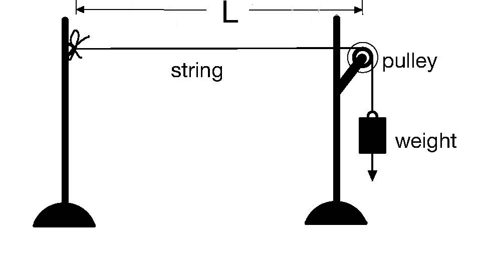
FIGURE \(5.\) Model of a string.
So far,
it is quite easy to imagine all that, but the question is, what are we
driving at by defining and focusing on those quantities? What we are
driving at is finding out
under what conditions will the string in question form standing waves when external energy, in the form of impulses, is imparted to that string?
This may seem as something far-fetched, but we are immediately reminded that it is standing waves that are the defining element when pondering about blackbody radiation. Therefore, we need to know the conditions under which these waves are formed, and the equation that governs them. As mentioned above, all our current exposé on blackbody radiation, following and critically examining the studies of Planck and all the rest of the students of blackbody radiation, revolves around this standing-wave-model of assembly of elementary participants in the blackbody radiation.
Why do we need a wave equation in order to derive the equation of the simple harmonic oscillator and not just use Hookes law, as was already done here?
As we saw, when speaking in a limited sense; that is, only about simple harmonic motion at a given frequency \(\nu\) and amplitude \(A\), the basic parameter to be reckoned with is the restoring force \(F = - \mathbb{k} x\), which one readily visualizes when thinking about a spring. When one stretches a spring, a force of resistance of the spring is felt in a direction opposite to the direction of stretching. This explains the negative sign in the formulation of the restoring force \(F = - \mathbb{k} x\). Also, for the same distance \(x\) of stretching (displacement), the resistance is greater, the greater the value of the spring constant \(\mathbb{k}\).
One may wonder why wasnt Hookes law, describing the restoring force \(F = - \mathbb{k} x\) of a string, enough to derive the equation of harmonic motion of a resonator of amplitude \(A\) and frequency \(\nu\), as was already done here? Well, of course, we could satisfy ourselves with that limited way of looking at wave motion when it comes to the special case of harmonic motion itself. However, the case of wave equation gives a general overview of the behavior of a wave modeled by a string, based on the balance of forces. This allows, for instance, finding the conditions for a standing wave. From Hookes law we learn limitedly what the temporal behavior (what the force of a spring extended to a given \(x\) is at a given moment) of a particular simple linear oscillator is. Combined with the spatial behavior of that same oscillator (that is, how kinetic energy changes when extending it) we, then, may derive what the expression for the overall energy of the simple harmonic oscillator iscf. here. By the way, that derivation also falls within the things in physics that cannot be disputed, and it must be kept in mind in any derivation having to do with simple harmonic oscillators. However, if we need more general conclusions, then we must resort to the wave equation.
The derivation of the wave equation that follows, is based on the balance of forces. FIGURE 6 shows a segment of a string for which the analysis of the forces will be made. The findings with respect to this segment of a string will represent the behavior of the entire string.
Now, we need to find out the resultant of the forces, \(\sum\limits_{i = 1}^{i = n} F_i\), acting on that segment, which, then, by Newtons second law, will equal \(m a\).
To not complicate things, we would at once note that the force of tension \(\mathcal{T}\) is acting normal (perpendicular) to the surfaces of the two ends (cut perpendicular to the extension of the string). Imagine, if the string, clamped onto two supports at a distance \(L\), is left alone. The two forces, equal in magnitude but opposing each other, will pull it equally, and the string will be straight. However, if the string is acted upon externally in the y-axis direction (upwards), the x-axis and y-axis components of the two opposing forces \(\mathcal{T}\!\!\!\), normal to the said surfaces, will be disturbed (while keeping \(\mathcal{T} = const\)), which we will immediately mark by observing their x-axis, \(\mathcal{T} cos(\theta)\) and \(\mathcal{T} cos(\theta + \Delta \theta)\), as well as y-axis, \(\mathcal{T} sin(\theta)\), and \(\mathcal{T} sin(\theta + \Delta \theta)\), components. This should be pretty obvious and self-explanatory from FIGURE 6. Therefore, we will not burden the discussion with further explanation of the trigonometry involved in this case.
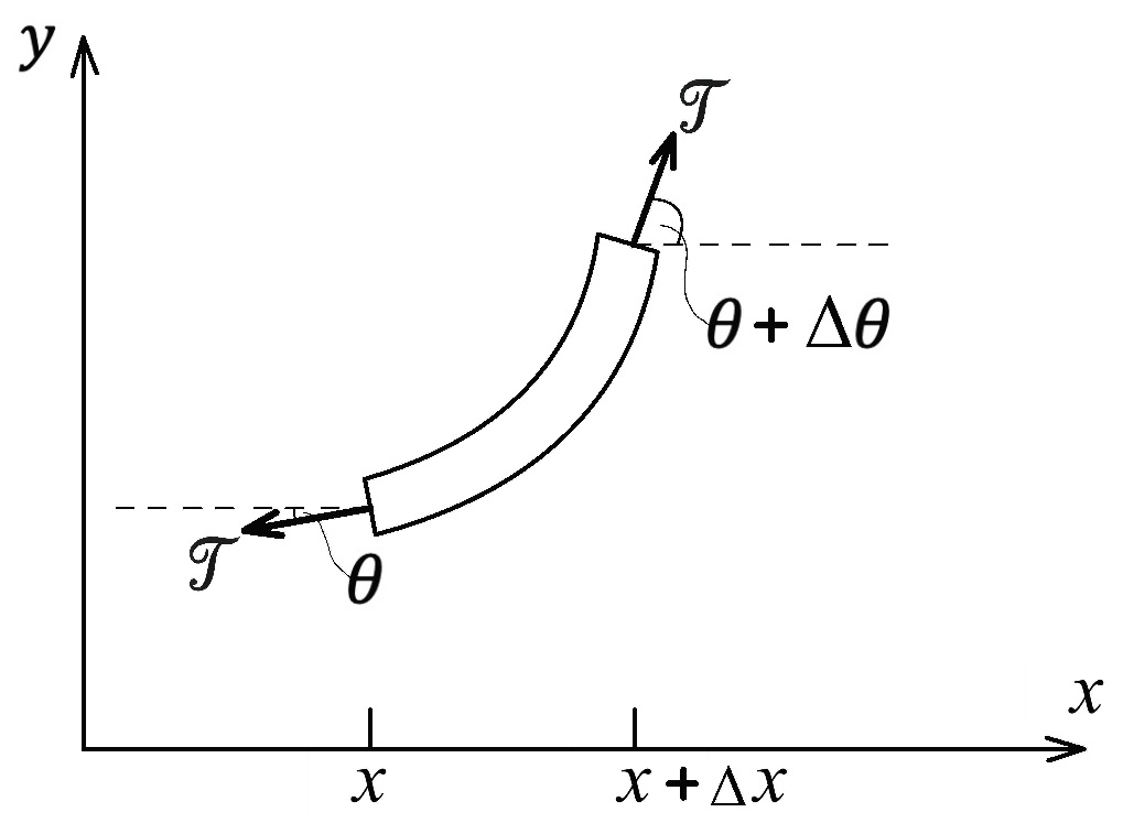
FIGURE \(6.\) Segment of a string.
The important thing now is to evaluate the sum of the forces along each axis; namely, x-axis and y-axis.
Thus, along the x-axis we have \begin{equation}\label{sumofTcomponentsalongxaxis} \sum\limits_{i = 1}^{i = 2} F_{x_i} = m a_x = \mathcal{T} cos(\theta + \Delta \theta) - \mathcal{T} cos(\theta), \end{equation}
while along the y-axis we have \begin{equation}\label{sumofTcomponentsalongyaxis} \sum\limits_{i = 1}^{i = 2} F_{y_i} = m a_y = \mathcal{T} sin(\theta + \Delta \theta) - \mathcal{T} sin(\theta). \end{equation}
Approximations
Here is an additional caveat, which we will have to keep in mind: The derivation will not only be for a small angle \(\theta\), but also for small change \(\Delta \theta\) of that angle.
Therefore, both \(cos(\theta) \approx 1\) and \(cos(\theta + \Delta \theta) \approx 1\), which means that eq.(\ref{sumofTcomponentsalongxaxis}), concerning the cosine component, is approximately zero.
Thus, we are relieved to deal only with the y-axis component; that is, with the sine component. In other words, we are finding ourselves lucky to deal only with the string moving up and down.
Further, we realize that having \(\theta\) and \(\theta + \Delta \theta\) small, allows also for another opportune approximation. This time the approximation concerns the sine part. Indeed, for small angles \(\theta\), we may write that \(sin(\theta) \approx \frac{sin(\theta)}{cos(\theta)}\), because, didnt we say, that for small angles \(\theta\), \(cos(\theta) \approx 1\). Therefore, \(sin(\theta) \approx \frac{sin(\theta)}{cos(\theta)} \approx tan(\theta) \approx \frac{rise}{run}\), which is, approximately, the slope of the observed segment of the string acted upon externally (if the string was not acted upon externally, the string will be flat because said slope will be zero). Written as a derivative, this slope of the segment of the string, acted upon externally, and represented by \(y(x, t)\), is \(\frac{\partial y}{\partial x}\). Although it is obvious, we will, nevertheless, note, that we are writing partial derivative (with curly \(\partial\), rather than straight \(d\)) because the function \(y(x, t)\) is a function of two variables, distance \(x\), and time \(t\), and we are keeping one of the variables, time \(t\), constant, while taking the derivative over the other variable, \(x\).
Therefore, we now may express the sum of y-axis component forces of the tension \(\mathcal{T}\), seen in eq.(\ref{sumofTcomponentsalongyaxis}) as \begin{equation}\label{vsSofT} \sum\limits_{i = 1}^{i = 2} F_{y_i} = m a_y = \mathcal{T} sin(\theta + \Delta \theta) - \mathcal{T} sin(\theta) = \end{equation} \begin{equation} \mathcal{T}\frac{\partial y}{\partial x} (\theta + \Delta \theta) - \mathcal{T}\frac{\partial y}{\partial x} (\theta). \end{equation}
Notice, \((\theta + \Delta \theta)\) and \((\theta)\) do not express multiplication or a functional dependence, but show for what angle the concrete derivative \(\frac{\partial y}{\partial x}\) is taken. In other words, \((\theta + \Delta \theta)\) and \(\theta\) signify for what value of \(x\) the derivative \(\frac{\partial y}{\partial x}\) is taken. Thus, the derivative signified by \(\frac{\partial y}{\partial x} (\theta + \Delta \theta)\) is taken for value of \(x\) equal to \(x + \Delta x\), while the derivative signified by \(\frac{\partial y}{\partial x} (\theta)\) is taken for value of \(x\) equal to \(x\). Therefore, instead of the above eq.\eqref{vsSofT} we may write \begin{equation*} \sum\limits_{i = 1}^{i = 2} F_{y_i} = m a_y = \mathcal{T} sin(\theta + \Delta \theta) - \mathcal{T} sin(\theta) = \mathcal{T}\frac{\partial y}{\partial x} (x + \Delta x) - \mathcal{T}\frac{\partial y}{\partial x} (x) \end{equation*} or \begin{equation*} \sum\limits_{i = 1}^{i = 2} F_{y_i} = m a_y = \mathcal{T} sin(\theta + \Delta \theta) - \mathcal{T} sin(\theta) = \mathcal{T} \left[ \frac{\partial y (x + \Delta x)}{\partial x} - \frac{\partial y (x)}{\partial x} \right]. \end{equation*}
Then, we can multiply the right side by \(\frac{\Delta x}{\Delta x}\), getting \begin{equation} \sum\limits_{i = 1}^{i = 2} F_{y_i} = \mathcal{T} \Delta x \left[ \frac{\frac{\partial y (x + \Delta x)}{\partial x} - \frac{\partial y (x)}{\partial x}}{\Delta x} \right]. \end{equation}
The expression in the brackets looks like a derivative at \(\Delta x \rightarrow 0\) within the brackets, but it is a derivative of a derivative; i.e., it is a second derivative. In other words \begin{equation}\label{balanceofyforces} \sum\limits_{i = 1}^{i = 2} F_{y_i} = \mathcal{T} \Delta x \frac{\partial^2y}{\partial x^2}. \end{equation}
One thing to understand here is the fact that, in order to have a curved segment, the resultant displacement along the y-axis must have a second spatial derivative. If the segment is straight, then \(\sum\limits_{i = 1}^{i = 2} F_{y_i} = 0\); that is, the two opposing forces of magnitude \(\mathcal{T}\) will compensate each other and the resultant force will be zero. Thus, the string must be curved, in order to feel a force along the y-axis.
Applying the known law (Newtons second law) to the obtained expression for resultant y-axis force
It is a basic law of physics, known as Newtons second law, that force \(F\) equals mass \(m\) times acceleration \(a\), \(F = m a\). Thus, on one hand, we have \(\sum\limits_{i = 1}^{i = 2} F_{y_i} = \mathcal{T} \Delta x \frac{\partial^2y}{\partial x^2}\) from eq.(\ref{balanceofyforces}), and on the other \(\sum\limits_{i = 1}^{i = 2} F_{y_i} = ma_y = m \frac{\partial^2y}{\partial t^2}\) from Newtons second law. More on the fact that this known form of Newtons second law represents only the temporal part of force will be discussed later (cf. section beginning here. Therefore, \begin{equation*} \sum\limits_{i = 1}^{i = 2} F_{y_i} = \mathcal{T} \Delta x \frac{\partial^2y}{\partial x^2} = ma_y = m \frac{\partial^2y}{\partial t^2}, \end{equation*}
where \(\frac{\partial^2y}{\partial t^2}\) obviously is the acceleration \(a\). We may reorder the above equation to obtain \begin{equation*} \frac{\partial^2y}{\partial x^2} = \frac{m}{\mathcal{T} \Delta x} \frac{\partial^2y}{\partial t^2}, \end{equation*}
then make the substitution \(\frac{m}{\Delta x} = \mu\), where \(\mu\) is linear mass density; that is, mass per unit length, and get \begin{equation}\label{prewaveequation} \frac{\partial^2y}{\partial x^2} = \frac{\mu}{\mathcal{T}} \frac{\partial^2y}{\partial t^2}, \end{equation}
which almost accomplished our goal, looking for the wave equation.
Dimensional analysis, revealing that \(\sqrt{\frac{\mathcal{T}}{\mu}}\) comprises velocity \(v\)
Now, we can observe a very interesting connection. It turns out that \(\sqrt{\frac{\mathcal{T}}{\mu}}\) is, in fact, \(\sqrt{\frac{\mathcal{T}}{\mu}} = v\). Doesnt this resemble the natural angular frequency \(\sqrt{\frac{k}{m}} = \omega\) of a simple harmonic oscillator, which we saw earlier here, eq.(\ref{omegasquaredeqaltokoverm}), where \(k\) is the spring constant (for simplicity, here we use \(k\) instead of \(\mathbb{k}\) because here there is no danger of mixing it up with Boltzmanns constant)? In both cases, at play are properties of the object undergoing periodic motion\(v\) (together with \(\mathcal{T}\) and \(\mu\)), and \(\omega\) (together with \(k\) and \(m\)). The quotient \( \frac{\mathcal{T}}{\mu}\), seen in eq.(\ref{prewaveequation}), and therefore of interest to us, the quotient we see within the formula \(\sqrt{\frac{\mathcal{T}}{\mu}}\) this section started with, is expressed dimensionally as \(\left[ \frac{N}{\frac{kg}{m}}\right]\), or \(\left[\frac{N \ m}{kg} \right]\), where \([N]\) is \(\left[\frac{kg \ m}{ s^2}\right]\). This results in \(\left[\frac{N}{\frac{kg}{m}}\right] = \left[ \frac{kg \ m}{\frac{kg}{m} s^2}\right] = \left[\frac{m^2}{s^2}\right]\), which are the dimensions of \(v^2\). Thus, instead of \(\frac{\mathcal{T}}{\mu}\), we may write \(v^2\), substituting in eq.(\ref{prewaveequation}) \(\frac{\mu}{\mathcal{T}}\) with \(\frac{1}{v^2}\) obtaining finally the wave equation itself, describing the vertical displacement of the string modeling a wave. We saw above that the horizontal displacement is \(0\), and therefore does not apply here; in other words, the vertical displacement fully describes the state of the string.
The wave equation itself
Thus, the sought for wave equation is as follows \begin{equation} \frac{\partial^2y}{\partial x^2} = \frac{1}{v^2} \frac{\partial^2y}{\partial t^2}. \end{equation}
Notice, the wave equation shows the connection between oscillations in space with the oscillations in time, the vertical displacement fully describing these oscillations. What kind of an equation this is and what and how its solutions are found is explained shortly. It is a wave equation because its solutions, the functions that satisfy it, are equations of periodic phenomena.
Speaking of velocity \(v\) of the wave, consider thisfrequency \(\nu\) is how many times per second the crest of the wave passes through a given point. Notice, in this case counting is vertical because, as said, the string in this case is undergoing only vertical displacement. Imagine that only one crest passes through that point in one second, replaced by another crest the next second. There is, however, a distance, wavelength \(\lambda\) between these two crests, which is, say \(1[m]\). Then, the speed of the wave in this case will be \(v = 1\left[\frac{m}{s}\right]\). The last formula also explains why \(v\) is given by the product of \(\lambda\) and \(\nu\), and not, say, by their quotient. Well, thats easy to figure out. Velocity \(v\) is expressed by meters per second and this can only come as a result of multiplying \(\lambda\) and \(\nu\).
Now, suppose the frequency \(\nu\) has risen to 5 crests per second passing through the point in question. Then, in order to keep the same velocity \(v = 1\left[\frac{m}{s}\right]\), the wave must decrease its wavelength \(\lambda\) to \(0.2 [m]\), so that \(v = \lambda \nu [m] \left[\frac{1}{s}\right] = 0.2 \times 5\) would give the same \(v = 1\left[\frac{m}{s}\right]\).
Thus, while frequency \(\nu\) of the wave is how many crests of the wave pass through a given point per second, it makes a difference if the distance between crests is short or it is long. If the distance between crests is long, then, although the frequency is the same, much longer distance will be passing through the point per unit time. Therefore, the velocity of the wave will be higher. Thus, in order to keep the velocity the same when the distance between crests becomes greater, we need to decrease proportionally the number of crests that pass through the point per second. Thus, because the speed of light is \(c = const \left[\frac{m}{s}\right]\), then the longer the \(\lambda [m]\), the lower the \(\nu \left[ \frac{1}{s}\right]\) will be, so that \(\lambda \nu [m] \left[ \frac{1}{s}\right]\) of that wave would stay the same \(c = const \left[\frac{m}{s}\right]\); that is, \(c = \lambda \nu\).
In a standing wave, although it is intuitively easier to understand frequencyfrequency will amount to how many times per second the standing wave will reach a given antinodethe passing distance through the antinode is hard to imagine. However, a standing wave also has a wavelength, and that is the distance between the antinodes. Therefore, the number of forming antinodes per second will correspond to the number of wavelengths per second, and the argument turns into the above argument concerning traveling waves.
Solving the wave equation
Now, weve reached the point which is the reason for this whole exercise of deriving the wave equation. Having the equation itself, we need to find what its solutions are for the conditions we are interested in; that is, we need to know what the wave equation solutions are, such that they would comprise standing waves. To begin with, the wave equation is a differential equation, a partial differential equation of the second order. Solution of a differential equation, unlike an ordinary algebraic equation, whose solution comprises finding a value or values which satisfy it, the solution of a differential equation is a function or a family of functions which satisfy it. The functions satisfying a differential equation may be many, but they can be limited in number if the physical problem imposes initial and boundary conditions. Herewith, we will deal with the boundary conditions. This pertains to our concrete example modeling wavesthe string. In other words, we seek solutions \(f(x)\), which will ensure that at the two ends of the string, where the string has been clamped to two immovable supports; that is, \(f(0)\) and \(f(L)\), are equal to zero for all times.
In the usual case, a case such as this one, finding the solutions of a second order partial differential equation is not straightforward. What is done, is resorting to guesswork, and if we are lucky, we may fall upon the right solution.
Thus, the beginning steps are to review what we have at hand:
we have length \(L\) of the string
we know that the string is clamped at the two ends, and that, in order
to prevent it from sagging we have transferred one of its ends over a
pulley and have attached a weight to it with the goal to impart force
of tension \(\mathcal{T}\) to the string.
we know that the string has mass density \(\mu\)
we already know that the equation describing the string motion when
external periodic thrust is applied to it is
\(\frac{\partial^2y}{\partial x^2} = \frac{1}{v^2}
\frac{\partial^2y}{\partial t^2}\), where \(v =
\sqrt{\frac{\mathcal{T}}{\mu}}\).
Now, having all this, the only thing we can do is resort to guesswork.
The so-called normal mode solutions
In view of our goalexploring the conditions for obtaining of a standing waveour guesswork will be directed towards obtaining the so-called normal mode solutions. These are the only solutions that will ensure that standing waves are resting (have zero displacement) at any time at the points where the string is clamped. Standing waves may also have other resting points along its extension. All these are normal modes of the string.
Now, here we must think a littlethe solution, the wave we are seeking, must move up and down in time; that is, the amplitude of the wave that would be a solution should change up and down in time, but, that up-and-down motion will not occur, at least at the spatial values corresponding to the beginning, \(x = 0\), and the end, \(x = L\), of the string. Therefore, we, of course, must first think of a periodic function which changes its deflection \(y\) in time at the different \(x\) but at the same time be zero at any time at the beginning \(x = 0\) and at the end \(x = L\). A perfect function for this job is \begin{equation}\label{trialfunction} y(x, t) = f(x)cos(\omega t). \end{equation}
The cosine is chosen for convenience. Equally as well it might have been the sine function.
Now, that the function seen in eq.(\ref{trialfunction}) is suggested as the trial function, someone may wonder why the product \(f(x)cos(\omega t)\) of these two functions was proposed and not, for example, their sum \(f(x) + cos(\omega t)\). Well, no one is stopping anyone from trying \(f(x) + cos(\omega t)\) as the test function for the solution of the wave equation, as long as it can be proved that \(f(x) + cos(\omega t)\) is indeed a solution of the wave equation. It is not.
Before proceeding, there may be a need for a heads up regarding the test-function (if it indeed happens to be the solution to the wave equation, which it will, as will be shown). In the end, for our purposes; that is, for finding the conditions for a standing wave, we will only need the spatial part \(f(x)\) of the test-function \(f(x)\cos(\omega t)\). Furthermore, curiously, that spatial part \(f(x)\) of the compound function \(f(x)\cos(\omega t)\), we will present in a harmonic-oscillator-form which resembles the temporal part \(\cos(\omega t)\) of the test-function \(f(x)\cos(\omega t)\), but, in fact, is a function of the spatial coordinate \(x\) through using the characteristic velocity \(v = \sqrt{\frac{\mathcal{T}}{\mu}}\). Thus, in the end, as a heads up, we will find ourselves using the function \(A\sin\left(\frac{\omega}{v}x\right)\) to determine what the conditions for a standing wave are. In other words, what angular velocities \(\omega_n\) or, rather, what frequencies \(2 \pi \nu_n\) (because \(\omega = 2 \pi \nu\); the meaning of the important number \(n\) will become clear later) must be imparted to the string, in order for the string to exhibit standing waves. Of course, also as a heads up, finding these frequencies \(\nu_n\) will not be enough. We will further need to know how many of these frequencies exist in the studied enclosure, which will be a further task to fulfill. Have patience, and all these further tasks and conditions will be revealed.
Now we can plug that guessed function \(y(x, t) = f(x)\cos(\omega t)\) into the wave equation \(\frac{\partial^2y}{\partial x^2} = \frac{1}{v^2} \frac{\partial^2y}{\partial t^2}\) and see if it satisfies that equation: \begin{equation*} \frac{\partial^2(f(x)\cos(\omega t))}{\partial x^2} = \frac{1}{v^2} \frac{\partial^2(f(x)\cos(\omega t))}{\partial t^2} \end{equation*} Now, because the differentiation on the left of the equation is with respect to \(x\), holding \(t = const\), we get, on the left \(\frac{\partial^2 f(x)}{\partial x^2}\cos(\omega t)\). On the right of the equality, we hold now \(x\) constant and differentiate with respect to \(t\), getting on the right, after two times differentiating of the cos, \(-\frac{1}{v^2} f(x) \omega^2 cos(\omega t)\), or written together \begin{equation*} \frac{\partial^2 f(x)}{\partial x^2} \require{cancel} \bcancel{\cos(\omega t)} = -\frac{1}{v^2} f(x) \omega^2 \require{cancel} \bcancel{\cos(\omega t)} \end{equation*} \begin{equation}\label{resultofpluggingintheguessfunction} \frac{\partial^2 f(x)}{\partial x^2} = -\frac{\omega^2}{v^2} f(x). \end{equation}
Thus, the plugging in of our guess-function \(y(x, t) = f(x)cos(\omega t)\) (only the part \(f(x)\) of which is unknown, the other part is knownit is a cosine) into the wave equation \(\frac{\partial^2y}{\partial x^2} = \frac{1}{v^2} \frac{\partial^2y}{\partial t^2}\) led us to the above eq.(\ref{resultofpluggingintheguessfunction}).
Now, if we manage to find what the exact form of this unknown function \(f(x)\) might be, we would have managed to find the solution to the second-order partial differential equation (the wave equation) \(\frac{\partial^2y}{\partial x^2} = \frac{1}{v^2} \frac{\partial^2y}{\partial t^2}\).
Therefore, we begin scratching our heads and it suddenly dawns on us that the function \(f(x)\) could only be the spatial form of the function of the simple harmonic oscillator equation of motion, because only the function of the simple harmonic oscillator recovers its initial form after two times of differentiation. This is how we arrive at the equation of simple harmonic motion as the solution of the wave equation. However, those who are impatient to see what this simple harmonic oscillator equation exactly is, must hold on. It will be revealed shortly, depending on the conditions needed for it to describe a standing wave.
Conditions arising from the simple harmonic equation of motion solution for our concrete model
Now that we concluded that the solution to eq.(\ref{resultofpluggingintheguessfunction}) must be nothing other than the equation of the simple harmonic oscillator in its spatial form, let us see what conditions are needed for this equation to describe a standing wave.
Tricks used to determine what conditions the simple harmonic oscillator equation must obey, in order for it to describe a standing wave
In order to fulfill the task of finding the conditions which the simple harmonic oscillator equation needs to obey, for it to describe a standing wave, we must do a couple of chores.
Preparing the simple harmonic oscillator equation in a spatial formBefore dealing with what the value of the phase \(\phi\) of a standing wave must be, we will deal with the following problem. As has become obvious, the solution of eq.(\ref{resultofpluggingintheguessfunction}) must be the equation for an oscillator exhibiting simple harmonic motion. It was said above, however, that we need the spatial version of that equation, so that we can apply to it the boundary conditions, whereby \(f(x) = 0\) for \(x = 0\) and \(x = L\). However, this poses a problem. We are used to writing the equation of simple harmonic motion in its temporal form; that is, in terms of a function of time \(t\). This will not allow us to explore it at the boundary conditions for \(x = 0\) and \(x = L\), where the function \(f(x)\) is \(0\).
In order to overcome this problem and convert the usual simple harmonic motion equation expressed as \(f(t)\) into an equation of the simple harmonic oscillator as \(f(x)\), we apply the following trick. We saw that the square root of the ratio (quotient) of the constants of the string \(\mathcal{T}\) and \(\mu\) gives velocity; that is, \(\sqrt{\frac{\mathcal{T}}{\mu}} = v\). We can write the time-dependent simple harmonic oscillator equation \(f(t) = A \sin(\omega t + \phi)\), equivalently as the spatial; that is, x-dependent, simple harmonic oscillator equation \(f(x) = A\sin(\frac{\omega}{v}x + \phi )\) and ... Voila! ... we can treat spatially; namely, we can treat as the function of \(x\), the simple harmonic oscillator equation. This substitution is justified because \(\omega t = 2 \pi \nu t\) is, in fact, \(\frac{\omega}{v}x = \frac{2 \pi \nu}{ \sqrt{\frac{\mathcal{T}}{\mu}} } x = \frac{2 \pi \nu}{v}x = \frac{2 \pi \nu}{ \frac{\require{cancel} \bcancel{x}}{t} } \require{cancel} \bcancel{x} = 2 \pi \nu t\).
By the way, we should write again that equation explicitly. Here it is, \(f(x) = A sin(\frac{\omega}{v}x + \phi )\), for those who were earlier impatiently wondering what the exact form of that spookily mentioned earlier equation of simple harmonic motion, celebrated as the spatial solution of the wave equation, if theyve failed to notice it.
OK, now, after we are happily settled with representing the equation for the simple harmonic oscillator as a function of \(x\), we may proceed with the next chore, and see what the conditions must be for the existence of standing waves.
Determining the value of the phase \(\phi\)The first thing we are going to see under the boundary conditions \(f(0) = 0\) and \(f(L) = 0\), is that the phase \(\phi\) is \(0\). It is convenient now to work in terms of the spatial variable \(x\), isnt it?
OK. Now, these boundary conditions will first allow us to get rid of the phase \(\phi\) because \begin{equation*} f(0) = A\sin\left(\frac{\omega}{v} 0 + \phi \right) = 0 \end{equation*} \begin{equation} f(0) = A\sin(\phi) = 0. \end{equation}
The function \(\sin(\phi)\) is zero when \(\phi\) is zero. Of course, the function \(f(0)\), which is \(A sin(\phi)\) can be \(0\) if also \(A\) is \(0\), but that is trivial. The function \(f(0)\), which is \(A sin(\phi)\) can be \(0\) even for \(A \ne 0\) if \(sin(\phi) = 0\); that is, if \(\phi = 0\). In other words, in order to have a standing wave, the phase \(\phi\) must be \(0\). This is one of the conditions for having a standing wave, but it is kind of intuitively felt, boring, not comprising the pivotal conditions for our clamped string to exhibit standing waves. Therefore, we may take the condition \(\phi = 0\) at \(x = 0\) only as a detailnotice that for the determination that a standing wave must have \(\phi = 0\), we use only one of the boundary conditions; namely, \(y = 0\) at \(x = 0\). This is the commonplace part.
The interesting part follows when we explore what the conditions for a standing wave must be at the other end of the string, \(x = L\), where the function \(f(x)\) must also be zero.
Determining the interesting boundary condition
Now, once we have determined that in a standing wave the phase \(\phi\) must be \(0\) at \(x = 0\), the interesting part, as already said, comes when we explore the condition for a standing wave at the other end of the string \(f(L) = 0\), or \begin{equation*} f(L) = A\sin\left(\frac{\omega}{v} L + \phi \right) = 0. \end{equation*}
But, first of all, we already saw that the phase is \(\phi = 0\), so, that term goes, as a first step: \begin{equation*} f(L) = A\sin \left(\frac{\omega}{v} L \right) = 0. \end{equation*}
Besides, we already said that considering \(A =0\), in order for \(A\sin \left(\frac{\omega}{v} L \right)\) to be zero, is trivial, and therefore we will look for the other possibility for \(A sin \left(\frac{\omega}{v} L \right)\) to be zero (which would be the condition for having a standing wave); namely, by having the sine function be \(0\).
In other words, we will see under what conditions \(\sin\left(\frac{\omega}{v} L \right)\) would be zero. Now, here we encounter another trivial possibility for the studied term to be zeroin this case the term \(\sin\left(\frac{\omega}{v} L \right)\) would be zero if, trivially, \(\omega = 0\). This is not interesting, however, because, as said, it is trivial. Well, then, explore the case when \(\omega\) is not zero, \(L\) is not \(0\) and \(v\) is not \(0\). So, what do we do? Are we left without options, other than the trivial ones to have the conditions at the other end \(L\) of the string, for the string to exhibit a standing wave? Not at all, because we suddenly realize that the sine function has peculiar properties. It is periodic, therefore it is \(0\) not only when the angle, in this case \(\frac{\omega}{v} L\), is \(0\), but also when the angle \(\frac{\omega}{v} L\) is equal to \(\pi\), or to any integer number of \(\pi\). Consequently, the condition for the string to exhibit standing waves when clamped between two supports, is for the angle \(\frac{\omega}{v} L\) to be \begin{equation} \frac{\omega}{v} L = \frac{2 \pi \nu}{v} L = n \pi, \end{equation}
where \(n = 1, \ 2, \ 3 \ \dots\), called normal modes of vibration and \(v\) is velocity. In other words, our string can exhibit standing waves (this is enunciated in a different way by saying normal modes can exist) only at frequencies \begin{equation*} \nu_n = \frac{n \require{cancel} \bcancel{\pi} v}{2 \require{cancel} \bcancel{\pi} L} = \frac{n v}{2 L} = \frac{n \sqrt{\frac{\mathcal{T}}{\mu}}}{2 L}. \end{equation*}
or, for an electromagnetic wave, we have \begin{equation}\label{conditionfordtandingwavefrequency} \boxed{\nu_n = \frac{n c}{2 L}}. \end{equation}
This is the most important part, which is arrived at in the process of solving the wave equation. At that, recall, the conclusion in the form of eq.(\ref{conditionfordtandingwavefrequency}) was reached only by analyzing the part \(f(x)\) of the entire solution \(y(x, t) = f(x)\cos(\omega t)\), eq.(\ref{trialfunction}), to the wave equation.
Just for the recordThe entire solution \(y(x, t)\) of the wave equation
The entire solution (recall the trial function, eq.(\ref{trialfunction}), we successfully tested, consisted of a spatial \(f(x)\) term and a temporal \(\sin(\omega t)\) term) of the wave equation, a solution which will ensure (or corresponds to) standing waves is \begin{equation} y_n(x, t) = A\sin \left(\frac{\omega_n}{v}L \right)\cos(\omega_n t). \end{equation}
However, we give the general solution only for the record because we have already extracted the needed information, the needed conditions for the string to exhibit standing waves and those conditions are given by eq.(\ref{conditionfordtandingwavefrequency}).
The ultimate goal of the above exercisehow many are these \(\nu_n\) in the studied enclosure?
Now, that we have the allowed frequencies \(\nu_n = \frac{n \sqrt{\frac{\mathcal{T}}{\mu}}}{2 L}\), we ask ourselves, how many of these frequencies are present in the enclosure, the subject of our studysee FIGURE 3B. Instead of the total number of these frequencies in the enclosure, it will be easier to find their density (their number per unit volume). This we can do by finding the number of said frequencies in a thin spherical shell around the center of a coordinate system, having along its x, y and z axes the allowed (for a standing wave) numbers \(n = 1, \ 2, \ 3, \ \dots \ \).
Before proceeding, we must downgrade the expression for the permitted frequencies \(\nu_n = \frac{n \sqrt{\frac{\mathcal{T}}{\mu}}}{2 L}\) that are valid for any wave to be a standing wave, to describing these permitted frequencies concerning concretely only the electromagnetic waves. To do this, we must remember that \(\frac{\mathcal{T}}{\mu} = v^2\), therefore \(\sqrt{\frac{\mathcal{T}}{\mu}} = v\), which, considering that for electromagnetic waves \(v = c\), gives, finally, the expression \(\nu_n = \frac{n c}{2 L}\), pertaining to electromagnetic waves. This formula will be used from now on as the criterion indicating what allowed frequencies make the waves in our enclosure of length \(L\), standing waves.
Derivation of the part of the blackbody formula which exists in all cases (the inevitably classical part)
Having laid the foundations of the absolute criterion \(\nu_n = \frac{n \sqrt{\frac{\mathcal{T}}{\mu}}}{2 L}\) for any wave to be a standing wave, and especially the criterion \(\nu_n = \frac{n c}{2 L}\), whereby the general expression for velocity \(\sqrt{\frac{\mathcal{T}}{\mu}}\) is replaced by the speed of light \(c\), for an electromagnetic wave to be a standing wave, we now may move on and use that criterion to derive the indisputable part \(\frac{8 \pi \nu^2}{c^3}\) of the blackbody radiation expression in both the incorrectly arrived at (Plancks) \begin{equation} u = \frac{8 \pi \nu^2}{c^3} \frac{h \nu}{e^{\frac{h \nu}{k \theta}}- 1}, \end{equation}
and correctly derived (C. I. Noninskis) \begin{equation} \rho = \frac{8 \pi \nu^2} {c^3} \frac{\mathscr{h} \nu} {e^{\frac{\mathscr{h}\nu}{k T}}-1}. \end{equation}
As noted, we will use the symbol \(\rho\) for the spectral energy radiation density, instead of the symbol \(u\), the latter seen in Plancks paper\(^{1}\), in order to distinguish the spectral energy density formula \(\rho\) correctly derived by C. I. Noninski, on the one hand, from the formula, apparently similar but incorrectly arrived at by Planck, for the spectral energy density, denoted by Planck as \(u\), on the other hand. These two apparently similar formulae, the one for \(\rho\) versus the one for \(u\), have different physical meaningin fact, Plancks formula has no physical meaning at all, being the result of juggling with random formulae until the right function has popped up. Notice, while having no other choice, we resorted to guesswork when finding the mathematical solution of a second order partial differential equation, such approach is inapplicable when it comes to using a mathematical expression for describing physical phenomena. In the wave-equation case, we were faced with finding a solution of a mathematical expression, even if this solution were to abide by certain physical constraints. In a case of a physical phenomenon, such as blackbody radiation, it is not enough to find, through the methods of applied mathematics (curve-fitting) or through guesswork and adjustments, the shape of a mathematical formula, which recovers the experimentally found shape of a physical relationshipsomething that Planck did, to be shown shortly. In looking for a correct mathematical description of a physical problem, the formula that is arrived at must come about from physical principles. If this is the case, then the coincidence of the plot based on the derived formula following from physical principles, with the experimental plot, is the proof that the physical views, the understanding and explanation of the physical phenomenon, the theory proposed in deriving the formula, is correct. Thus, what science does is form a view which theoretically predicts what the run of the experimental curve will be. This is what C. I Noninski did (cf. here). He did not curve-fit a mathematical expression to conform to what has already been experimentally found, as Planck did.
The part \(\frac{8 \pi \nu^2}{c^3}\) of the entire blackbody radiation formula \(\frac{8 \pi \nu^2}{c^3} \frac{h \nu}{e^{\frac{h \nu}{k \theta}}- 1}\) gives the number (per unit volume) of the energy elements, to be defined below, characterizing all standing waves in a cavity. This number multiplies, in Plancks case\(^{1}\), an expression for the mean energy \(U\) of one oscillator as a function of the frequency \(\nu\). However, it is central to this book to emphasize the erroneous nature of what Planck endows this \(U \!\) with, not even being able to obtain the formula containing \(U\), wrongly imagining that it is the mean energy of the resonator. In contrast, C. I. Noninski arrives at a quantity having a clear meaning rooted in reality, proving that it is the mean heat \( \overline{\Rule{0em}{0em}{0em}\smash{\mathscr{q}}} \ \) per oscillator, which the resonators exchange among themselves. Thus, we will deal separately with \(\overline{\Rule{0em}{0em}{0em}\smash{\mathscr{q}}}\), which in C. I. Noninskis derivation has the correct physical meaning. C. I. Noninski\(^{11,12}\) (cf. the facsimile of C. I. Noninskis paper reproduced here) shows that the quantity denoted by Planck as \(U\!\!\), in fact, comprises the mean heat \( \overline{\Rule{0em}{0em}{0em}\smash{\mathscr{q}}} \ \) exchanged amongst the particles of a system. This we will discuss in the crucially important section entitled CLASSICAL DERIVATION OF THE SPECTRAL ENERGY DENSITY OF BLACKBODY RADIATION BY C. I. NONINSKI\(^{11,12}\), beginning here. The derivation shown in that section, a derivation which is the summit of this book with regard to the physical side of sustaining the correct, classical understanding of quantum mechanics, reveals the complete poverty of the concept that there is some new physics, other than the good old classical physics, behind the so-called quantum mechanics.
Basically, the goal which we will be pursuing in this first part of
our study, is
to
find an expression for a number.
More precisely, we will present here, for the convenience of the reader, the standard justification that the expression for that number is \(\frac{8 \pi \nu^2}{c^3}\). This exact expression, part of the central formula (as given in Plancks founding paper\(^{1}\), is contingently called in this book the pre-exponential factor. Said central formula; namely, \(u = \frac{8 \pi \nu^2}{c^3}\frac{h \nu}{e^{\frac{h \nu}{k \theta}}- 1}\), more precisely, its exponential factor (previously given this name here), is the very formula which was the initial confused stimulant to falsely announce the emergence of some new physics, known as quantum mechanics.
Notice, for a given wavelength \(\lambda\), comprising one hill and one valley, if observed at the moment when that wave has a maximum given amplitude, the energy corresponding to one period \(\mathbb{T}\) will comprise two set portions of energy for that wavesee FIGURE 7. So, alternating just one maximum and one minimum of a standing wave, will correspond to one portion of energy. We are not discussing here how much that portion of energy would be, but are only indicating the mere number of portionsin this case, as just said, one portion of energy, while in FIGURE 7 we see two alternating maximums and minimums, which corresponds to two portions of energy. This number is arrived at from classical physics alone, and has nothing to do with quantum mechanics.
However, within a length \(L\), which is one of the sides of the cavity modeling the blackbody radiation emitter, which we take, for simplicity, to have the form of a cube, Fig.3, there may be many maximums and minimums, depending on \(\lambda\). Indeed, there can be \(\frac{L}{\lambda}\) number of such portions of energy for a given standing wave having the wavelength \(\lambda\). When \(\lambda = L\) there will be two portions of energy corresponding to \(L\)cf. Fig.7. Now, notice, however, that not just any \(\lambda\) would result in a standing wave\(^{62}\)in order for a wave to be a standing wave, it is necessary that it stays put at the two ends of \(L\); that is, the wave must not go up and down at any of the two ends of the distance \(L\). Therefore, to just write \(\frac{L}{\lambda}\) will not give the number of energy portions that fit into the cavity with side \(L\).
Thus, we must look for a criterion which will tell us exactly what that wavelength \(\lambda\) of the wave must be, in order to have its portions of energy fit into the cubic enclosure with side \(L\). In other words, we need to answer the question: what is the \(\lambda\) of this particular wave, which will be a standing wave within the enclosure, secured at the two ends of that enclosure?
Obviously, because the standing wave is immovable at the two ends of the cubic box of edge length \(L\)the ends of the string are clampedthe minimal number of portions that can fit within the distance \(L\) must be a wave whose half-wave \(\frac{\lambda}{2}\) is equal to the length of the box edge \(L\). Indeed, the \(\lambda\) of every sinusoidal standing wave has 3 points which are immobilethe beginning, the middle and the end point. Therefore, the minimal fraction of a wave of wavelength \(\lambda\) which will contain points that will not be in motion, comprises the half of that wave of wavelength \(\lambda\); that is, the part of the sinusoidal wave having only the beginning and the middle immobile points. In other words, the minimal part of a standing wave of wavelength \(\lambda\) that can fit in the enclosure of edge length \(L\) and still maintain its quality of being a standing wave, is when that \(\frac{\lambda}{2}\) is equal to \(L\). However, obviously, a wave will continue to be a standing wave when 2 or 3 or any integer number \(l\) of half-wavelengths, \(\frac{\lambda}{2}\)s, of a given wave of wavelength \(\lambda\), are equal to the edge length \(L\). Thus, the condition for the wave to be a standing wave can be written formally as \(\frac{\lambda}{2} l = L\). Or, the criterion for the \(\lambda\) of the wave, rendering that wave a standing wave, is \(\lambda = \frac{2L}{l}\). Presumably, now that we have the allowed values of \(\lambda\) for a standing wave, we can go ahead and calculate the energy portions which each wave of allowed \(\lambda\) possesses. Thus, a standing wave which has \(\frac{\lambda}{2} = L\) will endow the enclosure with \(1\) portion of energy. When \(\lambda = L\), then the enclosure will be in possession of two portions of energy, and so on.
We can, however, express the number of these energy portions in the enclosure in a different, simpler way, aiming at reducing the problem to counting numbers (rather, numbers per unit volume). Because we are in physics we need to understand the physical meaning of the quantities, rather than use formal mathematics to come up with the result.
For
instance, instead of dealing with the \(\lambda\) itself, we can
express the number of these portions by counting the number of
antinodes, which we will denote as #antinodes, each antinode
representing one portion of energy. For instance, consider a standing
wave of wavelength \(\lambda\) equal to \(L\)in such a case there
will be \(2\) antinodescf. FIGURE
7.
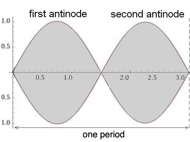
FIGURE \(7.\) One period of a standing sinusoidal wave. Imagine one wave going up and down, in the process swiping the grayed area. This standing wave exhibits two antinodes per period \(\mathbb{T}\). The two antinodes comprise the two maximums of the grayed area.
Therefore, the standing wave shown in FIGURE 7 corresponds to \(2\) portions of energy per period \(\mathbb{T}\). In other words, if the length \(L\) of the enclosure is equal to the wavelength \(\lambda\), that is, if \(\frac{L}{\lambda} = 1\) or \(\frac{L}{2 \frac{\lambda}{2}} = 1\), then the #antinodes will be \(2\frac{L}{\lambda} = 2\); if \(\frac{L}{\lambda} = 1.5\), then #antinodes \(= 2 \cdot \frac{L}{\lambda} = 2 \cdot 1.5 = 3\) and so on.
Now, if we need to express this #antinodes in terms of frequency, defining a standing wave in that particular cubic cavity having a length \(L\) of its edge, we get, beginning with the connection between wavelength and frequency \begin{equation*} \lambda \nu = c \end{equation*} \begin{equation*} \lambda = \frac{c}{\nu} \end{equation*} \begin{equation*} \frac{L}{\lambda} = \frac{\#antinodes}{2} \end{equation*} \begin{equation*} \frac{L}{\frac{c}{\nu}} = \frac{\#antinodes}{2} \end{equation*} \begin{equation*} \frac{\nu L}{c} = \frac{\#antinodes}{2} \end{equation*} \begin{equation}\label{sameconditionfordtandingwavefrequency} \boxed{\nu = \#antinodes \frac{c}{2L}}, \end{equation}
where #antinodes \(= 1, \ 2, \ 3, \ \dots \ \). As seen, the result, obtained in this heuristic way, dictating the conditions; namely, the value of \(\nu\), seen in eq.(\ref{sameconditionfordtandingwavefrequency}), for the string to exhibit standing waves, is the same as the result, eq.(\ref{conditionfordtandingwavefrequency}), obtained by solving the wave equation.
We
will find the expression \(\nu = \frac{c}{2L}\) #antinodes for the
allowed frequency to have a standing wave within the cubic enclosure
having the edge equal to \(L\), quite useful shortly, especially, for
#antinodes \(= 1\). As for the reordered expression for the
#antinodes, #antinodes \(= \frac{2L\nu}{ c}\), we may keep it in mind,
just for the record, to remind us what is meant when number of energy
elements carried by a standing wave is being inferred.
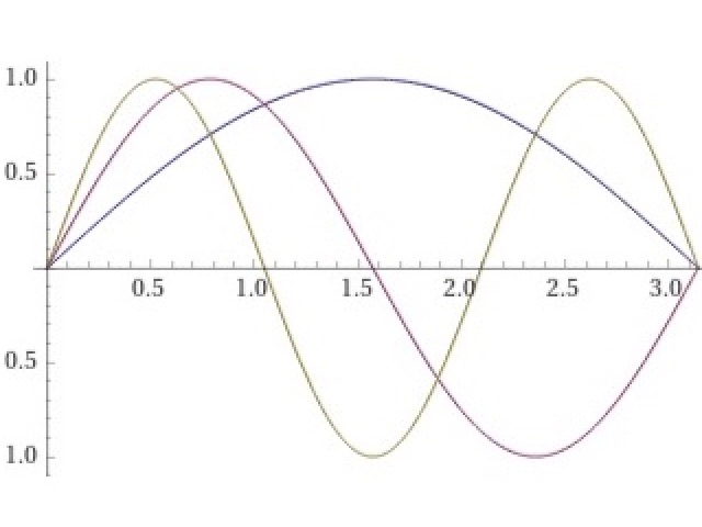
FIGURE \(8.\) Graph of three sinusoids.
Thus, when we know the #antinodes, we know how many individual complete energy bits we are dealing withas we just saw, one period \(\mathbb{T}\), or one wavelength \(\lambda\), consists of \(2\) such energy bits. You may refresh your memory as to how many bits of energy fit in an enclosure of length \(L\) by looking at FIGURE 8. We have already become savvy in discerning wavelengths \(\lambda\) and the individual bits \( \frac{\lambda}{2}\) that would fit within the cubic enclosure of edge length \(L\), so we will not be in much trouble discerning, as an exercise, that in FIGURE 8, whereby the length \(L\) spans the distance between the leftmost node and rightmost node, there is one wave having such a wavelength that only half of it, \(\frac{\lambda}{2}\) fits within the length \(L\). There is, however, another wave with such a wavelength, \(\lambda\), that has three halves, \(3 \frac{\lambda}{2}\), fit within the length \(L\). And, of course, we have the easiest example of a wave with such a wavelength \(\lambda\), whereby the entire period of that wave; that is, the \(2\) of its \(\frac{\lambda}{2}\)s fit within \(L\). Try it yourself, and see if you can convince yourself of that.
Density of the energy elements
So far, so good. Although somewhat lengthy, the derivation of the conditions for the standing waves was not difficult. Now, the next challenge; namely, determining the density of the energy elements in the enclosure of the blackbody studied by us, is somewhat more difficult. Notice, to simplify matters, in this book we are using our own terminology, defining energy elements corresponding to the #antinodes, not talking in terms of nodes and modes, as is usual in the standard literature.
As an aside, if we wish to use the term modes, each mode is characterized by a given set of #antinodes. Therefore, the #antinodes characterizes the frequency (the wavelength) as well as the mode. #antinodes defines \(\nu\) (or \(\lambda\)) through mode and vice versa. Keep in mind, every mode, consisting of a given #antinodes, is a carrier of a certain energy consisting of the corresponding number of individual energy elements, which corresponds to the frequency and the amplitude connected with that mode. Ultimately, however, we are interested in the #antinodes per unit volume for a given frequency for all entities, resonators (oscillators), in the system (this quantity may be called density of the #antinodes). Therefore, we write for the fundamental #antinodes \(= 1\), using the condition, eq.(\ref{sameconditionfordtandingwavefrequency}), for standing waves \(\nu = \#antinodes \frac{c}{2L}\), the following \begin{equation}\label{fundamentalfrequency} \nu_{_1} = 1. \frac{c}{2L}. \end{equation}
Notice the subscript \(1\) of the frequency \(\nu_{_1}\), indicating that it is the fundamental frequency, corresponding to the possibly lowest number of antinodes; namely, \(1\). Eq.(\ref{fundamentalfrequency}) shows the value of the fundamental frequency \(\nu_{_1}\) (frequency corresponding to the fundamental #antinodes \(= 1\)) only along one of the three axes of an imaginary coordinate system having frequency \(\nu\) along all axes. Consequently, if we want to express the condition for a wave to be a standing wave in the general case, then, in terms of \(3\)D frequencies, the virtual frequency-volume (the virtual frequency-volume is a contingent volume which differs from the real physical volume \(V = L^3\) of the enclosure) cannot be less than \begin{equation}\label{fundamentalfictitiousvolume} {\nu_{_1}}^3 = \left( \frac{c}{2 L} \right)^3 = \frac{c^3}{8 L^3} = const_{_1}^{\nu}, \end{equation}
(\(const_{_1}^{\nu}\) means the fundamental constant, corresponding to frequency \(\nu\)), whereby, luckily, \(c\), \(L\) and \(2\) are fixed. We will use this fictitious frequency-volume as the minimum frequency which we will overlay over a fictitious frequency-volume of a segment of a fictitious spherical frequency shell, in order to see how many times the elementary frequency-volume, eq.(\ref{fundamentalfictitiousvolume}), fits into that fictitious segment of a fictitious spherical shell. It is again to be emphasized that the appearance of frequency in the above formula is only as a part of calculating nothing other than just a number; namely, the number of energy elements. In more concrete terms, this number is going to be calculated in the following way (USEFUL REMINDERKeep in mindthe expression \({\nu_{_1}}^3 = \left( \frac{c}{2 L} \right)^3 = \frac{c^3}{8 L^3} = const_{_1}^{\nu}\), eq.(\ref{fundamentalfictitiousvolume}), abstractly represents \(1\) energy element):
Once we have the firmly established minimal frequency-volume; namely, \(\frac{c^3}{8 L^3}\), comprising the minimum (representing \(1\) energy element) firm condition for a wave to be a standing wave, we may divide the frequency-volume of any (representing any number of energy elements) thin spherical frequency-shell by that minimal frequency-volume, with the goal to establish how many such elementary (fundamental) volumes \( \left( \frac{c}{2 L} \right)^3 \) can fit in that spherical frequency-shell, thus obtaining the density of the elementary minimal conditions that determine the standing-wave status of a given blackbody cavity. Once we convince ourselves of what was just said, the rest is easy:
The volume of a thin spherical shellin terms of frequency \(\nu\) observed as the radiusis known from geometry courses as being \(4 \pi \nu^2 d\nu\).
Also,
because all the values observed are positive numbers, we will observe only \(\frac{1}{8}\) of the volume of the spherical shell, which gives us the volume of interest to be \(\frac{1}{8}4 \pi \nu^2 d\nu\),
and,
because we are exploring electromagnetic waves, there are, in fact, two mutually perpendicular standing waves. Therefore, the possible transverse polarizations of an electromagnetic standing wave are 2. If the wave is propagating along the x-axis, then it can only be polarized along the y and z axes (the in-between polarization can be reduced to these two polarizations). As a result, we must multiply the obtained volume by 2, to get \(2\frac{1}{8}4 \pi \nu^2 d\nu\)
Now, we are ready to divide the obtained frequency-volume of the part of the shell by the minimum (elementary, fundamental) frequency-volume which defines the condition for a wave to be a standing wave, considering also that the frequency-volume of the fundamental cell(the cell for the #antinodes \(= 1\)) for length \(L\), is \(\left( \frac{c}{2 L} \right)^3 = \frac{c^3}{8 L^3} = \frac{c^3}{8 V}\) (of course, for another length, say, length \(L_0\), the volume of the fundamental cellthe cell for the #antinodes \(= 1\)will be different): \begin{equation*} \#antinodes^{\nu} \ d \nu = \frac{2\frac{1}{8}4 \pi \nu^2}{\frac{c^3}{8 L^3}}d\nu = \frac{8 \pi L^3}{c^3}\nu^2d\nu \end{equation*}
or \begin{equation}\label{lockingexpression} \#antinodes^{\nu} = \frac{8 \pi L^3}{c^3}\nu^2. \end{equation}
Summary of the derivation of \(\frac{8 \pi L^3}{c^3}\nu^2\)
Let us see what we did here. We observed a part of an imaginary spherical shell with frequency considered as the radius. This is the mathematical side of the problem, which we may contemplate in any abstract situation. In order to bring the problem down to our case, limited to only allowed frequencies (determined by the dimension \(L\) of the enclosure), we calculated the mathematical expression for the imaginary volume of a spherical shell, comprising \(\frac{1}{8}^{th}\) of a sphere and calculated on the basis of the frequency considered as radius, and then divided the obtained expression by the minimally allowed frequency-based volume, also imaginary, corresponding to our case (corresponding to the dimension \(L\) of the studied enclosure). So, what we got is a mixture of linear dimensions and frequency, which, in its togetherness, provides us with just an allowed number of the individual energy elements as a function of frequency \(\nu\).
Therefore, if we now find an expression for the mean exchanging energy (heat) \( \overline{\Rule{0em}{0em}{0em}\smash{\mathscr{q}}} \) per oscillator as a function of \(\nu\) and view that \( \overline{\Rule{0em}{0em}{0em}\smash{\mathscr{q}}} \) as an individual energy element, then, for each \(\nu\) there will be a number, locked by the expression \(\frac{8 \pi L^3}{c^3}\nu^2\), eq.(\ref{lockingexpression}), indicating exactly what the number is of these energy elements, corresponding to the given \(\nu\), that comprise the entire system, which emits energy with that particular frequency \(\nu\). Multiplying the number \(\frac{8 \pi L^3}{c^3}\nu^2\) of the individual energy elements at a given frequency \(\nu\) by the mean value of an individual energy element (the mean exchanging energy (heat) \( \overline{\Rule{0em}{0em}{0em}\smash{\mathscr{q}}}\)) we will obtain the energy of blackbody radiation at a given frequency \(\nu\). Dividing that energy by the volume of the enclosure \(L^3 = V\) will result in the energy density \(\rho\) of blackbody radiation.
Here we will recall the fundamental distinction concerning the nature of the quantity \(U\), which Planck, aside from being incapable to derive an expression for it, incorrectly views as the mean energy possessed by one resonator and the physically consistent quantity \(\overline{\Rule{0em}{0em}{0em}\smash{\mathscr{q}}}\). Of course, had the quantity \(U\) been correct, we might have called it an energy element. However, it isnt and we will not discuss it further. Thus, if we are to refer to it at all, it would only be to repeat the statement for its wrongness.
Unlike Planck, who incorrectly views \(U\) as the constituent characteristic of the resonator, the correct, classical approach of C. I. Noninski views the energy element as a quantity \(\overline{\Rule{0em}{0em}{0em}\smash{\mathscr{q}}}\), detached from the resonator (oscillator) itself, comprising only the average energy (heat) which the resonator (oscillator) exchanges with other resonators. This is a pivotal difference, marking the boundary between the non-physical hallucinations, not even the result of a derivation, leading to the postulation of the impossible allowed and forbidden energy levels of the resonator itself (Planck), respectively, of the atom itself, on the one hand, and the entirely physically consistent derivation, based on classical physics (C. I. Noninski), describing quantities of energy (heat) exchanged outside the resonator or the atom, on the other hand.
In other words, the expression \(\frac{8 \pi L^3}{c^3}\nu^2\), eq.(\ref{lockingexpression}) (which we call throughout the book the pre-exponential factor), only clamps down how many elements (for the given \(\nu\)) are eligible to participate in calculating the overall energy, corresponding to that given \(\nu\).
Notice, also, that the frequency of the wave is not determined either by \(L\) or by #antinodes. That is, \(\nu = \#antinodes \frac{c}{2L}\), eq.(\ref{sameconditionfordtandingwavefrequency}), is only a criterion which tells us what the frequency must be in order for waves, having frequency for whatever reason of their own, would be standing waves. As for the parameter \(\nu\) in Plancks radiation formula, it is only a continuous running parameter (an independent variable), which, the pre-exponential factor grabs at every \(\nu\) and calculates the number of energy elements at that \(\nu\).
We, of course, do not fail to realize that only standing waves are of interest to us because they are the emitters of radiation.
Therefore, when we plot the energy of the blackbody radiation (not the energy densitydont fail to notice \(L^3\) in the numerator) (incorrectly) \(\mathcal{U} = \frac{8 \pi L^3}{c^3}\nu^2 \frac{h \nu}{e^{\frac{h \nu}{k \theta}} - 1} = f(\nu)\), respectively, (correctly) \(\mathscr{P} \, \, = \frac{8 \pi L^3}{c^3}\nu^2 \frac{\mathscr{h} \nu}{e^{\frac{\mathscr{h} \nu}{k T}} - 1}\) as a function of \(\nu\), we are only plotting the connection between the pre-exponential factor, which is in essence the criterion, and the exponential factor, which is the mean exchanging energy (heat).
By the way, it is immediately evident that if we need the expression for the energy density, \(u\), in Planck\(^{1}\) \begin{equation} u = \frac{8 \pi \nu^2}{c^3} \frac{h \nu}{e^{\frac{h \nu}{k \theta}}- 1}, \end{equation}
an expression which came about as a result of juggling with flawed formulae, and the properly derived energy density, \(\rho\), of blackbody radiation in C. I. Noninski\(^{11}\) \begin{equation} \rho = \frac{8 \pi \nu^2} {c^3} \frac{\mathscr{h} \nu} {e^{\frac{\mathscr{h}\nu}{k T}}-1}, \end{equation}
we must divide the expression for the energy of the blackbody radiation, \(\mathcal{U} = \frac{8 \pi L^3}{c^3}\nu^2 \frac{h \nu}{e^{\frac{h \nu}{k \theta}} - 1}\), respectively, \(\mathscr{P} \, \, = \frac{8 \pi L^3}{c^3}\nu^2 \frac{\mathscr{h} \nu}{e^{\frac{\mathscr{h} \nu}{k T}} - 1}\) by the volume \(L^3 = V\).
ADDENDUMDoes the pinhole color change when the size of the cavity becomes larger?
Now, we may get slightly curious as to what the comparison between the spectral energy (not energy density) distribution might be in two blackbody cavities made from the same material but different in size. We must see if there would be any difference in the position of the maximum in the \(\mathscr{P} \, \, -\nu\) plot.
Thus, we must let go tentatively of the frequency \(\nu\) as a running parameter and focus on finding what parameter might really be responsible for the effect, say, change of color, of the size of the enclosure. Superficially, it may appear that, indeed, the parameter \(L^3\) in the pre-exponential factor of energy (not energy density \(\rho\)) \(\mathscr{P} \, \, \) might affect the color coming from the pinhole. It may occur to us that the size of the enclosure determined by \(L^3\) may have something to do with the color of the pinhole because, was it not that there was an intimate connection between \(L\) and the frequency \(\nu\), frequency \(\nu\) actually determining the color. Thus, changing of \(L\) might be thought of as a factor changing the color of the pinhole. This must be checked by looking at the formula \(\mathscr{P} \, \, = \frac{8 \pi L^3}{c^3}\nu^2 \frac{\mathscr{h} \nu}{e^{\frac{\mathscr{h} \nu}{k T}} - 1}\).
Inspecting
the formula, we realize what the role of \(\nu\) is. Although \(\nu\)
is continuous for the entire formula, we realize that it is the
pre-exponential factor that divides, at every \(\nu\), the volume of
the imaginary primary frequency volume into the volume of the fraction
(one-eighth) of the infinitely thin spherical shell formed by the
frequency-radius. Therefore, at every \(\nu\) there is a particular
number which multiplies the exponential part \(\frac{\mathscr{h}
\nu}{e^{\frac{\mathscr{h} \nu}{k T}} - 1}\). That is why we said that
we must observe the pre-exponential and the exponential factor in
conjunction with each other. Consequently, the only conclusion we can
draw from the expression of energy (not of energy density)
\(\mathscr{P} \, \, = \frac{8 \pi L^3}{c^3}\nu^2 \frac{\mathscr{h}
\nu}{e^{\frac{\mathscr{h} \nu}{k T}} - 1}\), is that upon changing the
magnitude of \(L^3\) (changing the size; namely, the volume \(V =
L^3\), of the blackbody cavity), the only thing that would change is
the brightness of the emission of the pinhole, but not its color. The
change of \(L^3\) does not change the position of the spectral energy
distribution curve maximum along the \(\nu\)-axis, a change of
position which, if it took place (but it didnt), would have caused
change in color of the pinhole. The change of \(L^3\) only affects the
number of the energy elements for a given \(\nu\); that is, the height
of the spectral energy distribution curve but not the position of its
maximum determining the color. This explanation was added for those
who might wonder if the change of cavity size might affect the color
of a pinhole at a given temperature \(T\), knowing that blackbody
cavities of the same size but made of different materials display the
same color of the pinhole at a given \(T\), despite their outer
contraption being of a different color. Of course, as seen from FIGURE
9, at a given temperature \(T\), the pinholes of two
different-sized enclosures, even made from the same material, will be
of different brightness. As seen from FIGURE
9, however, the position of the maximum at the same \(T\)
remains the same, the color of the pinhole remains the same. Shift of
the maximum occurs only upon changing of \(T\). This is the already
commented on Wien displacement law here.
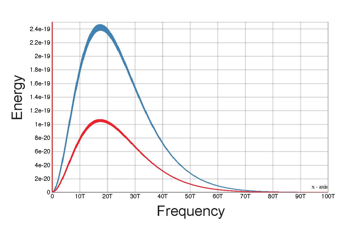
FIGURE \(9.\) Energy as a function of frequency for two blackbody cavities made of the same material but of different size at \(T = 298K\).
ADDENDUMWhy doesnt average energy \(kT\) per resonator, referring to the whole ensemble, apply to the individual constituent resonators equally?
The answer to the above question consists in noticing that Rayleigh and Jeans make an error (wrongly claiming ultraviolet catastrophe in classical physics) in their derivation of the controversial part of the blackbody formula (recall from eq.(8) in Plancks paper\(^{1}\), that the part \(\frac{8 \pi \nu^2}{c^3}\) of the formula is an absolute truth of nature, which we are deriving in this book here and here, while the form of the quantity \(U\) is the controversial part). They incorrectly ascribe to every single particle the average energy \(kT\) per each individual particle, while the reality is that because the individual particles themselves have different energies (different velocities), the groups of particles having the same velocity have average energies different from \(kT\)the truth is that the quantity \(kT\) per particle is derived for the entire assembly of the studied particles as a whole.
The
number of particles as a function of energy obeys an almost
bell-shaped velocity-distribution curve (in fact, more resembling
asymmetric Poisson distribution curve having a trailing right part).
Furthermore, a subsequent fact must also be noticed. This subsequent
but pivotal fact to appreciate, in pondering about all matters of
radiation, is that
although, in principle, the individual particles differ in their
energy (velocity), nevertheless, a greater portion of these particles
falls within the region around the average energy \(kT\), as seen in FIGURE
10. The number of resonators participating in the ensemble,
having energy greater than (or less than) \(kT\), falls steeply with
the increase (respectively, decrease) of the energy.
Thus,
surmounting the mean energy \(kT\), which is actually the point of our
concern, becomes exceedingly less likely with the increase of energy
(with the increase of \(\nu\)). In fact, a lower and lower number of
particles have energy exceeding \(kT\)consider the curve on the right
side of the maximum seen in FIGURE 10.
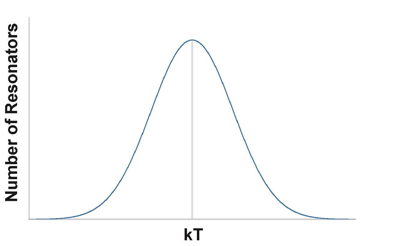
FIGURE \(10.\) Gauss distribution of the number of resonators plotted against energy. The figure shows that the number of resonators having energy greater that the mean energy \(kT\) drops fast with the increase of energy. The more realistic distribution is Poisson distribution with trailing right side of the curve. Gauss distribution is considered here for simplicity. It gets across the same idea.
This
means that when observing the radiation energy density distribution as
a function of frequency (which determines energy) of a set of
resonators residing in a blackbody cavity, we must expect a maximum of
that radiation energy. As we advance to higher and higher frequencies
of radiation, the maximum of energy will be overcome and the run of
the curve will begin sloping downthe resonators radiating at higher
frequencies (having higher energies) become ever lower in number with
\(\nu\), and their role in the overall energy becomes less and less
pronounced. The expected maximum is indeed seen in FIGURE
12 in the curve drawn according to Wiens distribution law and,
better yet, in the curve plotted according to Plancks distribution
law. The latter agrees the best with the experimental data such as
those of Lummer and Pringsheim, FIGURE
11.
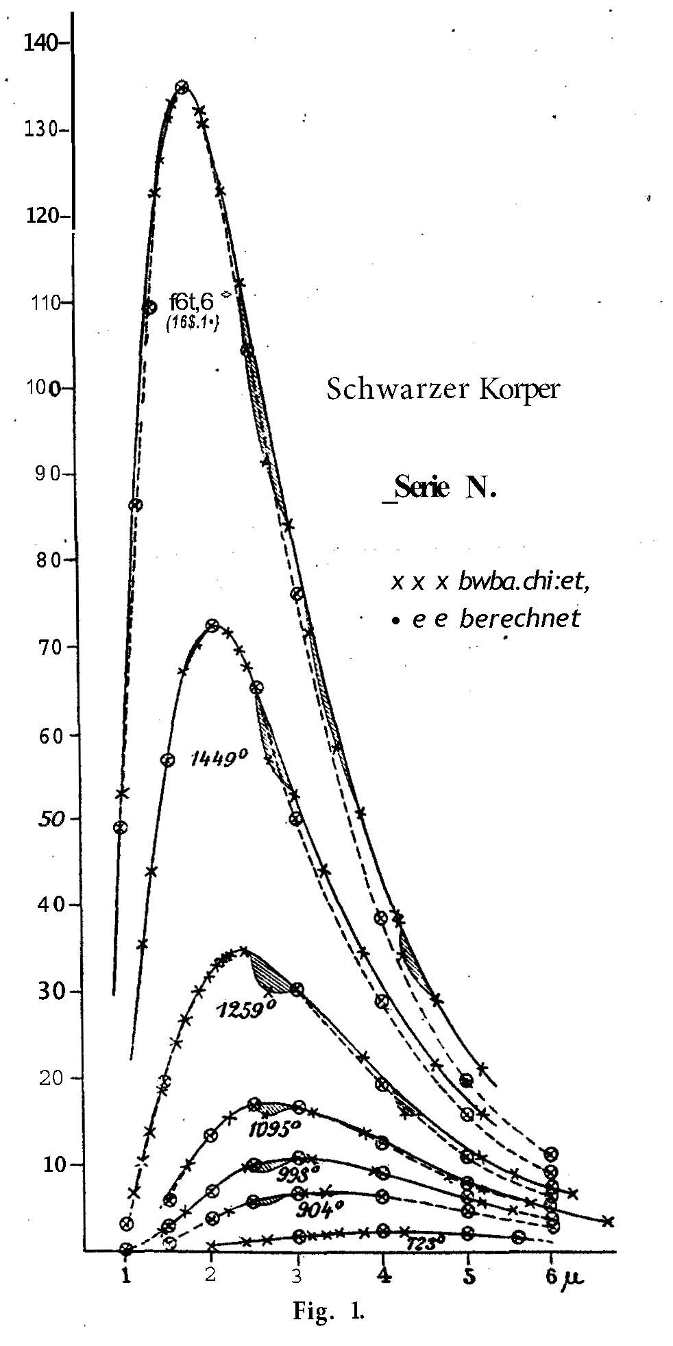
FIGURE \(11.\) Original plot from Lummer and Pringsheims paper.
On top
of it, Rayleigh and Jeans law plot is way off of all the experimental
values. Even worse, Rayleigh and Jeans curve shoots up into infinity,
instead of going through a maximum, with the increase of frequency
\(\nu\). The reason for that catastrophe, indeed, known as
ultraviolet catastrophe, was already discussedRayleigh and Jeanss
law does not provide for the obvious fact that individual molecules
have energies (velocities) different from \(kT\), and, even more
importantly, the energies exceeding the average energy \(kT\) are
possessed by fewer and fewer number of resonators, as the frequency
(energy) of these resonators increases beyond \(kT\). In Wiens,
better yet, in Plancks law, the infinite increase of energy density,
which the factor \(\frac{8 \pi \nu^2}{c^3}\) in eq.(8) of ref.\(^{1}\)
implies with the increase of frequency \(\nu\), is curbed by the ever
decreasing factor \(u\), also seen in eq.(8) of ref.\(^{1}\),
which in Wiens and, in effect, in Plancks formula, has an
exponential factor, steeply decreasing with frequency \(\nu\). The
opposition of the factor \(U\) to the increase of energy due to the
factor \(\frac{8 \pi \nu^2}{c^3}\) grows with the increase of
frequency \(\nu\), until that opposing factor begins to predominate,
finally suppressing the curve asymptotically toward zero at high
frequencies \(\nu\).
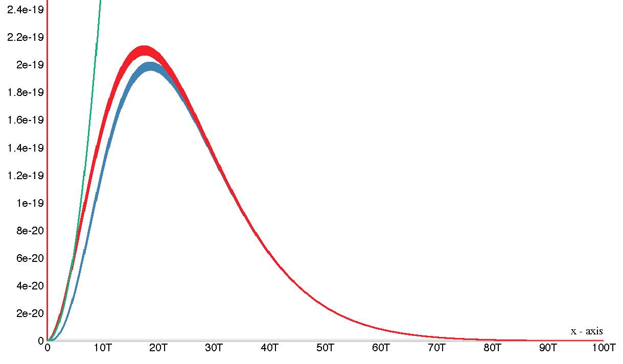
FIGURE \(12.\) Blackbody radiation curvesspectral energy density \(u\) (Plancks notation) plotted against frequency \(\nu\) at 298K. Curves with a maximum plotted from left to rightaccording to Plancks distribution law \(u = \frac{8 \pi \nu^2}{c^3}\frac{h \nu} {e^{\frac{h \nu}{k \theta}}- 1}\), and according to Wiens distribution law \(u = \frac{8 \pi \nu^2}{c^3}e^{-\frac{h \nu}{k \theta}}\). In order to fit the Rayleigh law \(u = \frac{8 \pi \nu^2}{c^3}kT\) into the graph, the value of the pre-exponential factor \(\frac{8 \pi \nu^2}{c^3}\) had to be decreased two orders of magnitude.
Here is a code to plot the above curves in websites such as https://mauriciopoppe.github.io/function-plot/ 6.1806445*10^(-58)*x^3*(1/(exp(x*1.6104751*10^(-13))-1)), Planck.
\( \large \mathbb{THE \ PHYSICAL \ PROBLEMS} \) \( \large \mathbb{OF \ QUANTUM \ MECHANICS} \)
A possible way of deriving the ideal gas law
We will begin these notes with an emphasis on the so-called ideal gas law (universal gas law), in view of its importance in theoretical science, far greater than is usually appreciated, despite its otherwise prominent ubiquitousness in science courses, especially in the courses of various branches of chemistry.
The ideal gas law, known by every good first-year student taking courses in chemistry, reads for \(1\) mole, almost as a mnemonic: \(PV = RT\). The meaning of the quantities participating in this law will become clear shortly.
The main thing to remember when deriving the ideal gas law is that, no
matter what mathematics we choose to use, we would not be able to
derive it mathematically had there not been the empirical discoveries
of the laws of Boyle, Charles and Avogadro, regarding the connection
between, respectively,
pressure \(P\) and volume \(V\) of the ideal gas at constant absolute temperature \(T\); that is, \(PV = const\) (Boyles law)
volume \(V\) and absolute temperature \(T\) at constant pressure \(P\); that is, \(\frac{V}{T} = const\) (Charles law)
and that
\(1\) mole of an ideal gas occupies a volume of 22.4L at STP (Standard
Temperature and Pressure, usually 25\(^{\circ}\)C (298K) and \(1\)atm)
(Avogadros law)
Once we know the above empirical relations, it is easy to write the following equations, considering also that \(V = V(P,T)\), or, spelled out in wordsvolume \(V\) is a function of pressure \(P\) and temperature \(T\). In other words, volume is a function of two variables \(P\) and \(T\). If we want to write the full differential of volume, we need to employ partial derivativestake the derivative of \(V\) with respect to one of the variables, keeping the other variable constant, and then take the derivative of \(V\) with respect to the other variable, keeping the first variable constant. What was said becomes immediately clear when it is written symbolically \begin{equation}\label{fulldifferentialofvolume} dV = \left( \frac{\partial V}{\partial T} \right)_P dT + \left( \frac{\partial V}{\partial P} \right)_T dP. \end{equation}
Eq.(\ref{fulldifferentialofvolume}) is open to some small modifications, then comparison with the stated empirical laws of Boyle and Charles follows.
Firstly, we will divide both sides of the equality in eq.(\ref{fulldifferentialofvolume}) by \(V\): \begin{equation}\label{fulldifferentialofvolumedividedbyv} \frac{1}{V}dV = \left( \frac{1}{V}\frac{\partial V}{\partial T} \right)_P dT+ \left( \frac{1}{V}\frac{\partial V}{\partial P} \right)_T dP. \end{equation}
The expressions within the parentheses can be treated the same way derivatives of functions of a single variable are treatedwell, when the second variable is held constant, the function remaining is only a function of one variable, isnt it? The subscripts at the bottom of the parentheses only indicate constancy of the other parameter and that does not interfere with the fact that we, in actuality, are taking derivatives, within the left and right parentheses, of functions of one variable only. Therefore, we may recall now that the simple relation concerning the first derivative of a logarithm is \(\frac{d \ln x}{dx} = \frac{1}{x}\), respectively, \(d \ln x = \frac{1}{x}dx\), or presented the way it will serve us better in the above equation: \(\frac{1}{x}dx = d \ln x\). Therefore, we may rewrite eq.(\ref{fulldifferentialofvolumedividedbyv}) as \begin{equation}\label{lnfulldifferential} d \ln V = \left( \frac{\partial \ln V}{\partial T} \right)_P dT + \left( \frac{\partial \ln V}{\partial P} \right)_T dP. \end{equation}
The expressions in the parentheses obviously yield, in a similar fashion, \(\frac{d \ln y(x)}{dx} = \frac{1}{y(x)} \frac{d y(x)}{dx}\), if we need to reassure ourselves that eq.(\ref{lnfulldifferential}) can bring us back to eq.(\ref{fulldifferentialofvolumedividedbyv}). Anyway, these are details which become obvious after taking some time to figure them out.
The next step is to substitute in eq.(\ref{lnfulldifferential}) the empirically obtained laws. Actually, we will now take the logarithm on both sides of the equality of each law. Thus, we have, after rearranging and taking the logarithm on both sides of Charles law \(\frac{V}{T} = const\) \begin{equation*} V = const \cdot T \end{equation*} \begin{equation*} \ln V = \ln const + \ln T, \end{equation*}
and, once we have the expression for \(\ln V\) (dont forget, presented to us empirically), we can at once calculate the first term in eq.(\ref{lnfulldifferential}) \begin{equation*} \left( \frac{\partial \ln V}{\partial T} \right)_P = \frac{\partial \left( \ln const + \ln T \right)}{\partial T} = \end{equation*} \begin{equation} \frac{\overbrace{ \partial \ln const}^\text{0} }{\partial T} + \frac{\partial \ln T}{\partial T} = \frac{\partial \ln T}{\partial T} = \frac{1}{T}. \end{equation}
From Boyles law \(PV = const\) we get by the same token \begin{equation*} V = \frac{const}{P} \end{equation*} \begin{equation*} \ln V = \ln const - \ln P, \end{equation*}
and the second term in eq.(\ref{lnfulldifferential}) becomes \begin{equation*} \left( \frac{\partial \ln V}{\partial P} \right)_T = \frac{\partial (\ln const - \ln P)}{\partial P} = \frac{\partial ( - \ln P)}{\partial P} = - \frac{1}{P}. \end{equation*}
Therefore, eq.(\ref{lnfulldifferential}) becomes \begin{equation*} d \ln V = \frac{1}{T} dT - \frac{1}{P} dP \end{equation*} \begin{equation*} d \ln V = d \ln T - d \ln P \end{equation*} \begin{equation*} d \ln V - d \ln T + d \ln P = 0, \end{equation*}
which, when assembling the logarithms, becomes \begin{equation*} d \ln \left( \frac{PV}{T} \right) = 0, \end{equation*}
and because zero can only be the differential of a constant, we get \begin{equation*} \ln \left( \frac{PV}{T} \right) = const, \end{equation*}
and because only a constant under the logarithm can result in a const, then the quantity \(\left( \frac{PV}{T} \right)\) itself is a constant, so finally, \begin{equation} \frac{PV}{T} = const. \end{equation}
Now, once we get to this point, allowing us to write \begin{equation} \frac{P_1V_1}{T_1} = \frac{P_2 V_2}{T_2}, \end{equation}
we may choose standard conditions, say, volume of \(1\) mole of ideal gas \(V = 22.4L\) at STP (Standard Temperature and Pressure), temperature \(T = 273K\), and pressure \(P = 1atm \), and that will result in the following value for the constant, which we denote by \(R\): \begin{equation} R = \frac{22.41 \times 1}{273.15 \times 1} = 0.082 \left[ \frac{L \ atm}{K \ mole} \right], \end{equation}
which, converted in \(\left[ \frac{J}{K \ mole} \right]\), having in mind that \(1L \times 1atm = 101.325 J\), gives \begin{equation} R = \frac{22.41L \times 101.325}{273.15} = 8.313 \left[ \frac{J}{K \ mole} \right]. \end{equation}
More accurate value of \(R = 8.314 \left[ \frac{J}{K \ mole} \right]\) is obtained if a more exact number \(v_m = 22.413969545014L\) of the molar volume of the ideal gas at STP is used. This is how the ideal gas law \(PV = RT\) for \(1\) mole of gas is arrived at, remembering the convention we adopted, for uniformity, that in this we will use upper case \(V\) to denote molar volume.
Boltzmanns constantThe derivations connected with blackbody radiation involve a constant known as Boltzmanns constant \(k\). It has a direct connection with the gas constant \(R\), \(R = Nk\), and, similarly, comes essentially from combining Boyles law, Charles law and Avogadros law, all of these empirical laws characterizing different aspects of the ideal gas, resulting, for any number of moles \(n\), in \begin{equation}\label{reorderedidealgaslawtoshowBoltzmannk} PV = nRT = \frac{N_{tot}}{N} {Nk}T = N_{total}kT, \end{equation}
where \(P\) is the pressure of the ideal gas, \(V\) is the volume of the ideal gas, \(N_{tot}\) is the total number of the molecules of the ideal gas, \(N\) is the Avogadro number, 6.022\(\times 10^{23}\), \(n\) is the number of moles of the ideal gas, \(T\) expressed as Kelvin temperature \([K]\), is the absolute temperature, \(R = Nk\) is the universal gas constant for \(1\) mole, expressed in \(\left[\frac{J}{K} \right]\), and \(k\) is Boltzmanns constant, also expressed in \(\left[\frac{J}{K} \right]\) for \(1\) molecule.
Resolution of the conflict between the ideal gas law and the equipartition theoremmean energy is \(\frac{3}{3}kT = kT\), not \(\frac{3}{2}kT\)
We must begin by pointing out that the needed correction, consisting of the derivations in this preparatory section, are new to science and cannot be found in the standard texts. This section introduces the reader to the basic notion of mean energy of a system containing an ideal gas, but also corrects an actually unrecognized conflict between how classical thermodynamics, as opposed to statistical thermodynamics, treats this mean energy.
Thus, now we want to get out of the way in this context as well, although it was already specially talked about (cf. here) the important matter of the average energy \(kT\) per particle (of an ideal gas, of course), when it pertains to the entire system of particles, while noticing that the individual particles (or groups of particles) themselves always have mostly various velocities \(v\); that is, the average energy of a group of particles having the same velocity \(v\) being different from \(kT\), or will be \(kT\) only as an exception.
It may not hurt to repeat the aboveas will be emphasized again later, \(kT\) is not the average energy when it comes to groups of particles within the system, each group having the same velocity \(v\) individually but different from the average velocity \(v\) of another group, as opposed to the average energy per particle when it pertains to the entire system of particles, where \(kT\) is the average energy per particle, calculated on the basis of all particles in the system, particles which otherwise individually always have mostly different average energies (average velocities \(v\)).
What was just discussed is what classical thermodynamics finds. When it pertains to the entire system of particles, always having different velocities \(v\) individually or in groups, that energy per particle classical thermodynamics finds to be \(kT\), rather than \(\frac{3}{2}kT\), as is the usual claim when the equipartition theorem in statistical thermodynamics is being considered. This usual claim of the statistical thermodynamics is in conflict with the ideal gas law, which is at the foundation of classical mechanics, together with the first and the second principle, and cannot be disputed (cf. eq.(\ref{reorderedidealgaslawtoshowBoltzmannk})). The clarity about the mean energy \(kT\) per particle, in a system of particles, helps to reassure us that when we talk about Boltzmanns distribution law applied to a system containing Avogadros number \(N\), the expression \(N_{greater} = N e^{- \frac{E}{kT}}\), given by Boltzmann for the number \(N_{greater}\) of particles, each having energy \(E\) greater than the mean energy \(kT\), is not in conflict with statistical mechanics (thus far claiming that the mean energy of the system is \(\frac{3}{2}kT\)). At the end of this section we will have a very satisfying feeling of unity, avoiding hidden loose ends. As a matter of fact, tying up loose ends, is the ongoing goal in every corner of this book.
Indeed, the detail we are going to deal with does not have an effect on the main conclusions regarding the physical problems calling for the defiance of the status of quantum mechanics as being a physical theory. However, it may still cause confusion along the way of understanding the physical grounds calling for the defiance, and that may slow down and cause uncertainty and shakiness in comprehending the matter.
The word is about the equipartition theorem, mentioned in connection with the early failed attempts to theoretically derive the experimentally observed spectral distribution of blackbody radiation energy density.
However, one should take a step back even into the very beginning of introducing equipartition of energy, and examine the viability of that theorem to begin with, when comparing it with an experimentally established law, such as the ideal gas law, which is an outgrowth of three laws discovered for ideal gas, referring to the constancy of each one of the three parameters, \(T\), \(P\) and \(V\), while changing the rest.
During this rumination, we encounter the following problem. When observing the ideal gas law for \(^{1}\) mole of gas \begin{equation}\label{idealgaslawpvnkt} PV = \underbrace{Nk}_\text{\(R\)}\ T \end{equation}
or \begin{equation}\label{idealgaslawpvrt} PV = RT, \end{equation}
we notice that both eq.(\ref{idealgaslawpvnkt}) and eq.(\ref{idealgaslawpvrt}) are expressions of energy of the gasthe temperature \(T\) (Kelvin temperature, [K]), expressed in units of Kelvin on the right side of these equations, cancels the temperature in the denominator of \(k\) \(\left[\frac{J}{K} \right]\), respectively, \(R\) \(\left[\frac{J}{K} \right]\), and what remains is the average energy in joules, respectively, of \(^{1}\) molecule and of \(^{1}\) mole of molecules of ideal gas.
Now, if the above were true, then there can be no other expression for the average energy of one molecule of ideal gas than the average energy given by the ideal gas law \begin{equation}\label{idealgaslawenergy} \overline{E}_{one \ molecule} = \frac{PV}{N} = kT. \end{equation}
In contrast to the above, the average energy \(\overline{E}_{one \ molecule}\) of one molecule of ideal gas, given by the equipartition theorem is \begin{equation}\label{equipartitionenergy} \overline{E}_{one \ molecule} = \frac{3}{2} kT. \end{equation}
As is seen from eq.(\ref{idealgaslawenergy}) and eq.(\ref{equipartitionenergy}), the ideal gas law and the equipartition theorem give two different results for the mean energy per particle regarding the same system. This is impossible. Of the two outcomes, only one, eq.(\ref{idealgaslawenergy}), is the correct answer to the question as to what the mean energy per particle is, assessed on the basis of the entire assembly of ideal gas particles.
Therefore, we need to observe separately, what the origin of the equipartition theorem is, on the one hand, and on the other, what the origin of the ideal gas law is. HINTAs far as the ideal gas law goes, it was already talked about. The origin of the ideal gas law is experimental, and therefore it takes precedenceany theoretical derivation pertaining to the relations between \(P\), \(V\) and \(T\), must lead to results in harmony with the ideal gas law.
From the above, it is obvious that what we need to do now is observe the derivation of the equipartition theorem, in order to ascertain that the equipartition theorem indeed abides by the ideal gas law. In the analysis of this theorem, the theorem at hand being a theoretical consideration, which in the end, has to prove that we may use relations between microscopic properties such as position \(x\) and velocity \(v\) of the individual molecules, in order to describe macroscopic properties such as \(P\), \(V\) and \(T\) of the gas, we have to be careful about two thingswhat the premises are for the theoretical assessment, on the one hand, and on the other, preserve the integrity of the derivation, and ensure the avoidance of circular arguments, known as the logical fallacy petitio principii.
Integrity of the derivation is maintained by handling only the microscopic properties and their relations in the attempt to derive the known relations between macroscopic quantities, not allowing the use of the known relations between macro-quantities in the process of proving that relations between macro-quantities can be derived through relations between micro-quantities.
In other words, in this derivation we must not use the ideal gas law because it is exactly the ideal gas law that we must derive out of microscopic quantities.
We will now present the premises just as they are given in the standard literature. Critical view of these premises will be postponed until after the standard presentation.
In the derivation of the equipartition theorem, the ideal gas observed has exactly the same limitations as the ideal gas described by the ideal gas lawrandomly moving, volumeless, non-interacting particles. In the case of equipartition theorem (unlike the usual cylinder with a piston, used when when discussing ideal gas in thermodynamics), these particles are enclosed in a cubic box of side \(L\). The particles, however, can collide elastically (without losing kinetic energy after the collision) with the walls of the cube, the duration of the collision itself being infinitely short.
Notice that in the above description of the ideal gas, there are additional elements to those that were had in mind when considering the ideal gas law. The old elements in the assumptions defining ideal gas, are the negligible volume of the particles compared to the total volume of the gas, the non-interaction, non-sticking together of particles when coming in contact, and no collision between them.
The new elements are, first, the cubic containerrecall ideal gas law observes the ideal gas in a cylinder with piston. New elements are also the velocity of the particles, their elastic collision with the walls and time between collisions. Such model appears very attractive for calculatory purposes, compared to the heuristic character of the macro-quantities world of classical thermodynamics. It may appear more attractive indeed, however, it must derive correctly the heuristic findings of classical thermodynamics, and that does not seem to be the case, at the time of this writing.
There are two tricky things that have to be initially understood, in order to have the follow-up derivation, standard as it is, be comprehended smoothly.
The first is the change of momentum (impulse) \(\Delta (mv)\), which is the difference of momentum \(-mv\) after the collision, equal in magnitude to the momentum before the collision with the wall, because of the collision being elastic, on one hand, and, on the other, the momentum \(mv\) before the collision with the wall. In other words, \begin{equation*} \Delta (mv) = momentum_{final} - momentum_{initial} = \end{equation*} \begin{equation}\label{impulse} \bbox[5px, border: 2px solid grey]{{ -mv - (+mv) = -2mv}} \end{equation}
While the just-discussed definition of \(\Delta (mv)\) is plausible, the second, the notion of time between collisions, involving the length \(L\) of cubes edge, and considering the round trip of the particle from the moment of colliding with the wall in question to the opposite wall, and then back to the wall in question, may be the subject of discussion as being too crude a model. Of course, it is clear that since collisions with the walls are elastic, and the particle does not change the magnitude of its momentum after the collision with the wall, then, upon impinging upon the opposite wall and the follow-up retracting from it, allows the particle to arrive at the initial wall unaffected. Knowing the velocity \(v\) of the particle and the double distance \(L\) it has traveled back and forth, the time between two successive collisions with the studied wall is expressed at once as \begin{equation}\label{timebetweencollisions} t = \frac{2L}{v}. \end{equation}
Now, aside from the fact that such a model requires infinite bouncing back and forth of every particle, it is even harder to imagine how particles moving, albeit in a straight line, but in different directions, would all begin their trip from one corner of the cube to the diametrically opposite corner, so that their x, y and z-components will travel the distance \(2L\) each, between two successive collisions with the wall at hand.
If we want to simplify matters and observe every particle moving only along one of the three axes, then, because of the random character of motion, the particles moving along x-axis will be only \(\frac{1}{3}\) of all moving particles. This is a very important observation because it eliminates the need to multiply the motion of a particle along the x-axis by \(3\) in order to cover the motions of the particles along the other two axesy-axis and z-axis.
Thus, when we write the force of Avogadros number \(N\) of particles on the wall, it will be enough to express only the change of momentum \(\Delta (mv)\) over time \(t\) of one particle along the x-axis, and then multiply that force by the total number \(N\) of particles, accounting in this way for the other \(\frac{2}{3}\)-rds of the particles, keeping in mind that there is no preferred axis-direction along the x, y and z-axis: \begin{equation}\label{expressionforf} F = \frac{\Delta (mv)}{t}, \end{equation}
which, combining eq.(\ref{impulse}) and eq.(\ref{timebetweencollisions}) obtains the form (neglecting the minus sign and the subscript \(x\) of velocity) \begin{equation*} \bbox[5px, border: 2px dotted grey]{ F = \frac{2mv}{\frac{2L}{v}} } \end{equation*} \begin{equation}\label{incorrectforce} \bbox[5px, border: 2px dotted grey]{ F = \frac{mv^2}{L} }, \end{equation}
and, because the surface area \(A\) of the wall is \(L^2\), we have for the pressure on the wall of all \(N\) particles \begin{equation*} \bbox[5px, border: 2px dotted grey]{ P =\frac{NF}{A} = \frac{N\frac{m\overline{v^2}}{L}}{L^2} } \end{equation*} \begin{equation*} \bbox[5px, border: 2px dotted grey]{ P = \frac{Nm\overline{v^2}}{L^3} } \end{equation*} \begin{equation*} \bbox[5px, border: 2px dotted grey]{ P = \frac{Nm\overline{v^2}}{V} } \end{equation*} \begin{equation*} \bbox[5px, border: 2px dotted grey]{ PV = Nm\overline{v^2} }, \end{equation*}
where \(\overline{v^2} = \frac{v_1^2 + v_2^2 + v_3^2 + \dots + v_N^2}{N}\) is the average of the squares of the velocities of all the \(N\)-number of molecules. In terms of kinetic energy \(\mathcal{E} = \frac{1}{2}m\overline{v^2}\), therefore, \(m\overline{v^2} = 2\mathcal{E}\), the only energy characterizing a monoatomic ideal gas, even after correcting the standard derivation for the 3-axes error, it can be written as \begin{equation}\label{avenmktheory} \bbox[5px, border: 2px dotted grey]{ \frac{PV}{N} = 2\mathcal{E} }. \end{equation}
However, according to the ideal gas law, \(\mathcal{E}\) is \begin{equation}\label{avenidealgaslaw} \frac{PV}{N} = \mathcal{E}. \end{equation}
Now, this is the moment to clearly spell out that, despite the comparison we make between the eq.(\ref{avenmktheory}) and eq.(\ref{avenidealgaslaw}) for the purposes of showing the discrepancy, no substitution from the ideal gas law must take place in the expression derived along the lines of the molecular-kinetic theory. The only thing that must happen at this point, is to explain away the discrepancy between eq.(\ref{avenmktheory}) and eq.(\ref{avenidealgaslaw}), by considering that eq.(\ref{avenidealgaslaw}) is the correct law, as being a law arriving from experiment.
So, there must be a problem somewhere in the premises of the molecular-kinetic derivation.
LOCATING THE PROBLEMThe problem is in eq.(\ref{impulse}), in which the change of momentum prior to and after the collision of the particle with the wall, is presented. However, what we are interested in
is not what the change of momentum is of the particle itself, as eq.(\ref{impulse}) expresses, but what the change of momentum is of the point where the particle hits the wall (if we really intend to use momentum of the particle to describe the pressure on the wall)are we not interested in what the pressure experienced by the wall is?
Therefore, the momentum at the point of the wall where the collision takes place, prior to the collision, is 0, while, the particle colliding transfers momentum \(mv\) to that point after the collision. Therefore, the change of momentum of the point where the particle hits the wall is \(\Delta (mv) = mv - 0 = mv\). As a result, we will replace in the equation defining force, eq.(\ref{expressionforf}); namely, \(F = \frac{\Delta (mv)}{t}\), the just obtained corrected expression for \(\Delta(mv)\); namely, \(\Delta (mv) = mv - 0 = mv\), after which eq.(\ref{expressionforf}) acquires the form \begin{equation*} F = \frac{mv}{\frac{2L}{v}} \end{equation*} \begin{equation} F = \frac{mv^2}{2L} , \end{equation}
and, because the surface area \(A\) of the wall is \(L^2\), we have for the pressure on the wall of all \(N\) particles \begin{equation*} P =\frac{NF}{A} = \frac{N\frac{m\overline{v^2}}{2L}}{L^2} \end{equation*} \begin{equation*} P = \frac{Nm\overline{v^2}}{2L^3} \end{equation*} \begin{equation*} P = \frac{Nm\overline{v^2}}{2V} \end{equation*} \begin{equation*} PV = N\frac{m\overline{v^2}}{2}, \end{equation*}
where \(\overline{v^2} = \frac{v_1^2 + v_2^2 + v_3^2 + \dots + v_N^2}{N}\) is the average of the squares of the velocities of all the \(N\)-number of molecules. When it comes to the energy of ideal gas, the kinetic energy \(\mathcal{E} = \frac{1}{2}m\overline{v^2}\) is the only energy characterizing monoatomic ideal gas. Thus, the correct expression of the kinetic energy \(\mathcal{E}\), derived from the molecular-kinetic theory, \begin{equation}\label{correctavenmktheory} \frac{PV}{N} = \mathcal{E}, \end{equation}
now properly coincides with the expression for \(\mathcal{E}\) obtained from the ideal gas law \begin{equation} \frac{PV}{N} = \mathcal{E}. \end{equation}
This coincidence, finally, may allow us to consider that statistics-based molecular-kinetic theory has also derived that \begin{equation} \frac{PV}{N} = kT, \end{equation}
as the ideal gas theory in thermodynamics has it. Furthermore, if one needs to distribute the energy among the quadratic terms in the expression for energy, then \( \frac{1}{3}kT\), not \(\frac{1}{2}kT\), would be the energy corresponding to each degree of freedom in the case of a monoatomic ideal gas.
PHYSICAL CONSIDERATIONSWhen the particle hits the wall, although the particle retains the magnitude of its momentum after the impact due to collision being elastic, the wall, nevertheless, must experience an effect. Otherwise, considering a collision by the particle, in order to come up with an expression of the pressure (on the wall), will make no senseindeed, we are not studying the effect of the collision on the molecule of gas. What we are really studying is what effect the collisions of the gas molecules with the wall had on the wall.
MORE PLAUSIBLE EXPLANATIONBecause there will be immediate objections to the above picture, based on what an elastic collision means, we will tune up even further the picture leading to the correct derivation from molecular-kinetic theory of the mean energy of the ideal gas. Each molecule has a momentum \(mv\), which may symbolize the momentum of a particle hitting an imaginary wall of area \(A = L^2\). In order to also utilize the formula \(t = \frac{2L}{v}\), eq.(\ref{timebetweencollisions}), for the time between collisions, we can place the imaginary wall infinitely close to the physical wall of the cube.
This eliminates the coefficient 2 when assessing the change of momentum when the particle hits the imaginary wall, in order for this action to be qualified as pressure.
It should not be strange that we are observing matters in this way because even in the standard derivation, when change of momentum \(\Delta (mv)\) was discussed, it was the change of momentum before and after the impact of the particle itself that was discussed. Involving the wall and colliding with the wall has no effect in the standard derivation when it comes to the wall. However, in such a treatment, the momentum quantity is observed twice, which is incorrect.
In the new, correct, picture, the imaginary area \(A = L^2\) is characterized by 0 momentum when the particle was flying towards it before crossing it. The moment the particle crosses that imaginary area, we may say that the area has experienced change of momentum from 0 to \(mv\). Therefore, the change of momentum experienced by area \(A\) (it is the change of momentum of that area that we are interested in, not in the change of momentum of the particle) is \(mv\). This, correct, model, makes all the difference when it comes to deriving the average energy of ideal gas via the micro-quantities of the molecular-kinetic theory.
With this, we conclude one piece of discussing general considerations, noting that there will be other places in this book devoted to refreshers and review of known notions, and will begin discussing topics closer to home; that is, the controversial problems connected with quantum mechanics.
The importance of understanding thermal radiation and energy as a whole as a basis for resolving quantum mechanics non-scientific basis
Although it is made to seem ubiquitous and well-established beyond any prospect of challenging it, understanding the flawed basis of quantum mechanics and the necessity to abandon it, is crucial for all science. The beginning of this process in science, of defying the substituting of cold formalism for meaning, has its roots in thermal radiation, specifically in the analysis of the unresolved problems of blackbody radiation, having already presented the absolute truths regarding that radiation. Such analysis we will undertake in the section that follows, after which we will discuss the way to pull out of this dead-end. Returning to classical mechanics and developing classical mechanics is the only correct way to go, should we need to have science at all.
On a wider note, if we are to bring the conversation to the practical needs of the global politics of the day, those who are concerned with environmental issues and contemplate anthropogenic impact on climate change, should appreciate the significance of properly studying the matters of energy, in particular, for example, matters of energy connected with radiation. Therefore, it would make sense to take some time for studying the part of this book that follows, since, all that was said so far having more or less a preparatory character, what follows contains the bulk of what is wrong with the main ideas of contemporary science.
HITHERTO UNRESOLVED PARTS OF BLACKBODY RADIATION FORMULAPLANCKS PAPER
No discussion on the viability of quantum mechanics as science can take place without analysis of the 1901 Planck paper\(^{1}\), introducing the subject. For quantum mechanics, Plancks paper\(^{1}\), as problematic as it is, as shown below, has the same significance as the 1905 paper on relativity\(^{3}\), the latter being a complete, embarrassing failure (cf. my books Relativity is the Mother of All Fake News, Pathology of Relativity and Some Notes on General Theory of Science and No Great Reset as well as the proof here).
The first to show the failure of the physical principles of quantum mechanics, laid out by Planck in his 1901 paper\(^{1}\), was C. I. Noninski in his 1964 paper\(^{11}\) (cf. the facsimile here). Later, I published a number of papers showing the mathematical as well as logical problems, especially in the quantum mechanical postulates, rendering quantum mechanics non-science.
In this book, I go further than C. I. Noninskis critique of Plancks paper, showing the impossibility of the statistical premise for the derivation presented. This finding is crucial and leads to the dissipation, right from the beginning, of the idea that quantum mechanics has anything to do with science. In its immediacy and unequivocality of debunking, outright excluding the discussion of any further details pertaining to Plancks paper\(^{1}\), the rejection of quantum mechanics presented herewith much resembles the greatest rejection ever achieved in sciencethat of my debunking relativity in my book Relativity is the Mother of All Fake News(in this book, presented here)considering also the extent of its penetration into science and society.
Aside from the sheer illogical basis of quantum mechanics, what remains of it, is nothing other than misunderstood classical mechanics. Therefore, unlike relativity, which is catastrophically flawed, and therefore must leave science without a trace, quantum mechanics, luckily, has an outlet of salvation with classical mechanics.
Catastrophe of Plancks Paper
We must state outright, and without any hesitation, that Plancks paper falters as early as eq.(3) seen in ref.\(^{1}\), an equation reading \(S_N = k\,\!\log\,\! W\), which we will discuss fortwith. Plancks paper\(^{1}\), upon initially encountering it, gives as a first impression that it is quite detached anyway from what many of us have heard quantum mechanics to be. However, that is a sense that eventually may turn out to be unjustified, as happens so often when encountering new ideas in science. Alas, this time, that gut feeling failed to betray the novice.
After this discovery has been made, in order to see this now easily discernible scientific calamity, we will be aided by a facsimile, presented for convenience of the reader, beginning here, the English version of that 1901 Plancks paper\(^{1}\), still widely, albeit erroneously, considered seminal for physics.
At the beginning of that paper, Planck introduces the reader to what brought him to the thoughts he intends to develop further in his paper. Planck mentions several names, but this only touches the surface of the vivid atmosphere in those days regarding the problems of thermal radiation. As it turns out, witnessed by the arguments that follow, these problems are as actual and in need of immediate correction today, as they were in those days, not in the least because they are concerning not only physics, but also areas such as astronomy and other scientific disciplines, to say nothing about the major adverse ramifications these ideas had, and still have, on many other significant aspects of life. Therefore, those who opine that the fundamentals of quantum mechanics are a closed chapter are in for a big surprise.
Unfortunately, the ramifications of the flawed discipline of quantum mechanics went aggressively astray into a gigantic development of crippled ideas, which not only have no root in reality, but, in fact, are damaging society. This wrongness was dealt with in one stroke by C. I. Noninski with his 1964 paper\(^{11}\), which will be the source of continuous inspiration in this book, demonstrating that there is nothing unusual in quantum mechanics, neither are there any earth-shaking observations in physics, requiring radical change in our views about nature beyond the developments which the classical physics (classical physics is physics without relativity and quantum mechanics) would suggest. It follows from C. I. Noninskis paper\(^{11}\) that it is not classical physics to blame for being incapable of deriving the correct physical picture, in harmony with experimental findings, such as the run of the blackbody radiation curve. If anyone is to blame, it is the failure to correctly apply classical mechanics by the investigators who took the task upon themselves. Unfortunately, C. I. Noninskis paper is still unappreciated. That causes the massive persistence of deformed views in physics, science and all aspects of life, in general, slapping every so often the wrong idea that there is something otherworldly out there, which defies common sense and comprises an unthinkably weird reality.
Plancks influence on young scientists
Planck
had a great influence, and young scientists caught on to that and
furthered this iniquitous approach of doing science, eventually making
a name for themselves, while causing erosion of scientific thought and
thought in general, to this day. There was especially one of these
young fellows, whom one can almost hear saying
... wait ..., is that the
way science is done ... allowing for the illogical to be considered
logical and the unequal to be considered equal? Watch me ...
and he surpassed his authoritative teacher many times over. We will see below more than one example, created by this champion of the absurd.
Mincing no words in presenting one more of the important contributions of this bookthe unequivocal invalidating of the physical basis of quantum mechanics
As in
the previous books, where the overthrowing of relativity was
demonstrated right away, here, when it comes to debunking the physical
foundation of quantum mechanics put forth in Plancks paper\(^{1}\),
the circumstances again allow taking the bull by the horns. What will
be shown is one more, paradoxically, fortunate example of an extremely
rare opportunity to resolve promptly, yet rigorously and
unequivocally, not only a pivotal question of science, but a question
of historic significance. The arguments in question remove in one
stroke the claim that the genesis of quantum mechanics has physical
foundations, formed around blackbody radiation. This discovery, to be
presented in the following paragraphs, saves even the effort of the
otherwise correct critique by C. I. Noninski in his paper\(^{11}\),
who has failed to notice that one need not at all analyze the
threatening looking formula \(S = k \left\{ \left(1 +
\frac{U}{\varepsilon} \right) \ln \left( 1 + \frac{U}{\varepsilon}
\right) - \frac{U}{\varepsilon}\ln \frac{U}{\varepsilon} \right\}\),
from which, if we gullibly agree that it shows entropy \(S\) as a
function of \(U\), which Planck considers the vibrational energy
possessed by a resonator, it follows that when \(S\) is zero, the
quantity \(U\) will also be zero, and therefore \(U\) cannot be the
internal energy of the resonatoran observation, in fact, contained in
Plancks very paper\(^{1}\). Indeed,
paradoxically, Planck himself admits in \(\S1\) of his paper\(^{1}\),
while failing to heed his own admission, that
If amplitude and phase
both remained absolutely constant, which means completely
homogeneous vibrations, no entropy could exist and the vibrational
energy would have to be completely free to be converted into work.
This discrepancy between what Planck says in words and what he actually derivesnamely, considering that \(U\) is the vibrational energy of the resonator, which, according to the formula he derived would become zero when the entropy \(S\) becomes zero, although himself admitting in words that the internal energy (the vibrational energy \(U\) of the resonator) will not be zero when \(S\) is zero, because it would have to be completely free to be converted into workwas discovered by C. I. Noninski\(^{11}\).
The immediately seen catastrophic truth
However, even C. I. Noninski has failed to notice that the entropy formula \(S = k \left\{ \left(1 + \frac{U}{\varepsilon} \right) \ln \left( 1 + \frac{U}{\varepsilon} \right) - \frac{U}{\varepsilon}\ln \frac{U}{\varepsilon} \right\}\), which Planck thought he derived, makes no sense, let alone can that formula even be reached, because of the following simple, yet dramatic fact, obliterating the entire derivation attempt in Plancks paper\(^{1}\); namely, the fact that the entire derivation in Plancks paper\(^{1}\) is eliminated because Boltzmanns statistical formula \begin{equation}\label{Boltzmannstatisticalformula} S_N = k\, \log\, W + const, \end{equation}
used for that derivation, is a non sequitur, as far as the goal of the particular derivation in paper\(^{1}\) goes. In that formula, presented here as eq.(\ref{Boltzmannstatisticalformula}), \(W\) is considered the probability so that the \(N\) resonators together have the energy \(U_N\)\(^{1}\) (der Wahrscheinlichkeit \(W\) dafür, dass die \(N\) Resonatoren insgesamt die Energie \(U_N\) besitzen).
However,
the fact that the resonators together have fixed energy \(U_N\), is an
initial condition of Plancks derivation. It, being a definition and
an initial condition, is absolutely true by default. An absolutely
true definition enjoys 100% certainty. Its probability is unity.
Therefore, the probability that the resonators together have energy \(U_N\), is unity by default, which means that (after suitable determination of the additive constant) \begin{equation} S_N = k\,\!\log\,\!W = k\,\!\log\,\!1 = 0. \end{equation}
This is catastrophic for the derivation, and the entire paper\(^{1}\) must be abandoned at once, right at the outset, making the job of the analyst extremely easy. The story ends right here.
Final conclusion about Plancks paper\(^{1}\)
The only conclusion, after the fiasco shown above, at the onset of the derivation, consisting of the fact that \(S = 0\), is that Planck is unable to derive the spectral energy density of blackbody radiation \(u = \frac{8 \pi \nu^2}{c^3}\frac{h \nu}{e^{\frac{h \nu}{k \theta}}- 1}\), despite the superficial impression to the contrary by the deceitful appearance of having coherent derivational steps, an impression given for over a century that he has derived said formula. The deceitful appearance of derivational steps could mislead even C. I. Noninski, the critic who was able to unearth the problem later in this quasi-derivation, a disaster bound to happen anyway, because it is planted in the earliest premise of the pseudo-derivation. It is very important that the reader understand that. Because of the \(S = 0\) fiasco, any further postulation, including the famous postulation that \(\varepsilon = h \nu\), the cornerstone of quantum mechanics, is out of the question. It is simply not possible. Planck would not even be able to exercise in any way his inclination to postulate that \(\varepsilon = h \nu\). Quantum mechanics is dead before it was even conceived, which is proven in the very pages of its founding paper. Curiously, quantum mechanics fails in the very pages of its founding paper in the same way the theory of relativity fails and invalidates itself in the very pages of its founding 1905 paper which introduces it to the world.
On the criterion of validity of a derivation
Planck states that only experience is the criterion for the validity of the hypothesis that the entropy is expressed by Boltzmanns formula, in which the probability \(W\) is replaced by the number of complexes \(R\).
However, coincidence with experience may occur due to purely formal reasons, such as, being the result of using a particular suitable mathematical function, which can be established by curve-fitting alone, and curve-fitting does not amount to a scientific derivation. Therefore, coincidence between a formula and experience may be a purely formal coincidence, and may not necessarily reflect a correct understanding of the physical nature of the observed phenomenon. For instance, the exponential function, as such, in principle fits the data produced by studying many unconnected phenomena, but that fitting does not mean that their nature is the same. In fact, the nature of the phenomena described by an exponential function may be dramatically different.
Such formal coincidence, as is the case in ref.\(^{1}\) between the graph of a formula and the experimental graph, cannot be the criterion for the validity of derivation or even that a derivation has taken place at all, for that matter, but one must look for the underlying physical essence of the hypothesis.
In the studied case, the number of ways a given energy \(U_N\) is distributed amongst the given number \(N\) of resonators, can hardly be probability. For a given system the number of ways \(R\) of distributing the fixed amount \(U_N\) of energy, distributed amongst a fixed number \(N\) of resonators, is a constant.
Look at it this waywe saw above that Planck cannot even reach the point of talking about \(S\) and \(U\). However, even if we forget about this and proceed with Plancks derivation, it is seen that when Planck thinks that he derives \(S\) as a function of \(U\), he first must have apprehended what, indeed, this \(U\) is. Even if we go along with Plancks declared, in effect flawed, understanding of the nature of \(U\), even then the things dont jive. The value of \(U_N\) is fixed because \(U_N = NU\) is fixed, and therefore \(U_N = P \varepsilon\), is fixed, respectively\(P\) is the total number of available energy elements \(\varepsilon\), where \(\varepsilon\) is a single energy element.
Therefore, \(P = \frac{NU}{\varepsilon}\) is also constant, from which it follows that \(dS\) as well as \(dU\), are zero, which means that \(\frac{dS}{dU}\) is indeterminate. However, the intention to plug \(S\) into \(\frac{dS}{dU} = \frac{1}{\theta}\), is a defining step in the derivation, which, given the just stated facts, fails miserablythe derivation goes nowhere, even if we agree, for the sake of argument, that \(W\) is proportional to \(R\).
Hence, no matter whether or not the hypothesis agrees with experience, the derivation fails because Planck cannot even determine \(S\) and \(U\), let alone that \(S\) and \(U\) are constant, which leads to the above-seen indeterminacy. Someone may object that, after all, the formula obtained, no matter how formally, fits the experimental data. However, as already said, a solely formal adjustment of a formula to fit what is desired, is not enough at all for a derivation in physics to be correct.
Incidentally, checking with the concrete numbers given in ref.\(^{1}\), plugged into the expression for \(R\), can be used as an easy criterion indicating whether or not \(R\) can be considered as the probability so that the \(N\) resonators together have the energy \(U_N\)\(^{1}\) (der Wahrscheinlichkeit \(W\) dafür, dass die \(N\) Resonatoren insgesamt die Energie \(U_N\) besitzen).
Checking with the real numbers given in \(\S3\) of ref.\(^{1}\) makes matters worse for the proposed hypothesis, as already noted, because it is 100% certain that the \(N\) resonators together have the energy \(U_N\), since this is the condition of the problem, the default. Said probability, now denoted by \(R\) (put in the place of the probability \(W\)), must necessarily be of value \(1\). If \(R \ne 1\), then, the hypothesis that \(R\) is the probability so that the \(N\) resonators together have the energy \(U_N\)\(^{1}\), is unsustained. In the case at hand, when the concrete data are plugged in, \(R\) is not even equal to \(1\), as it must be. Therefore, \(R\) cannot be considered as probability. The hypothesis that \(W\) is proportional to \(R\) fails on this account as well.
As is obvious, the problem does not go away even if it is claimed that \(W\) is the probability so that the \(N\) resonators together have the energy \(U_N\)\(^{1}\) were an inadvertent error, while what Planck really meant was \(W\), respectively \(R\), represents the probability for a certain energy complex to be realized. \(R\) indeed gives the number of such complexes for a given \(N\) and \(P\). However, even in such a case, and even if we agree that the number of the equally probable complexes expresses some compound probability for the formation of such complexes, even under such correction, the number obtained for \(S_N\) will be a constant for the system under consideration. It is obvious, then, that the \(dS\) sought for, will be \(dS = 0\), to say nothing of the fact that \(dU\) will also be zero because \(U\) is defined in paper\(^{1}\) as the time average of the energy of one resonator (which is a constant) or simultaneous average of the energy of \(N\) identical resonators having frequency \(\nu\) (which is also a constant), hence \(\frac{dS}{dU}\) will be indeterminate, not equal to \(\frac{1}{\theta}\), as we already discussed above. This disables the possibility to derive the blackbody radiation formula in the way proposed in Plancks paper\(^{1}\).
Exposing the physical inconsistency of quantum mechanics is long overdue
The physical inconsistency of quantum mechanics should have been detected around the nineteen hundreds, right at these early stages of the attempt at advancing it as a legitimate science. That erroneous path of science should have been prevented, in order to avoid the dead-end in which science now finds itself.
Reiteration of fundamentals
We need to reiterate that no matter what technical progress there might be in perfecting experiment or elaborating on the mathematical machinery, all this will be in vain if the physical fundamentals are non-existent, as they are in the case of quantum mechanics, as was already exposed, and as will be revealed even further momentarily.
Of course, we must prominently note that nothing at all erroneous can match the so-called theory of relativity in its quality of being brazen absurdity (for proof cf. here, that has spread like the plague, engulfing a sizable part of humanity. The unmatched aggressive absurdity of relativity is never to be forgotten by anyone who cares about science, even if he finds comprehending the flawedness of another absurdity, such as quantum mechanics, difficult and over his head. Relativity allows understanding its absurdity by immediate inspection. Relativity invalidates itself on the very pages of its 1905 founding paper\(^{3}\) (for proof cf. here). This remark on relativity is necessary to be kept in mind, especially by those to whom high science feels like an insurmountable mountain, the mere thought of climbing it appearing unfathomable. The ease with which every person of average intelligence can discern the scientific poverty of the most important theory symbolizing contemporary science, relativity, smashes to smithereens any wall of protection which anyone would try to build around senselessness, in order to up its importance, wrapping it in mystery and exclusive, let alone elusive, specialness. More on the claptrap known as relativity is to come shortly.
The lost science, suppressed by consensus
Besides, it is useless to wait or rely on some they, who will clarify discrepancies, if such discrepancies are found. We should also not assume that there are no discrepancies only because no one else has yet reported such, and millions upon millions of pronounced scientists in the world have adopted a certain picture of nature, and a certain view about how things work. The essence of scientific exploration is such that one may be right and millions wrong. As a matter of fact, this is exactly what discovery issomeone finds something which millions have been oblivious to, failing to see it. Hence, no reassurance must be expected from the millions, in anticipation of recognizing a discovery. A discovery is identified based on its own merits and argumentation, not by consensus amongst others. Therefore, the more a claimed discovery relies on consensus, the less scientific it is. Notably, sometimes, wrong views persist for thousands of years, as happened with the Aristotelian views solely based on perception. Consensus about incorrect views, perceived as correct, has persisted for centuries.
Searching for absolute truths, as in relativity, allowing incurring of the final blow
The above discussion makes it imperative to once again draw some general conclusions regarding the theory of science, as was already done, detaching ourselves from the concreteness of the topic at hand.
This analysis follows the approach applied in my three previous books Relativity is the Mother of All Fake News, The Pathology of Relativity and Some Notes on the General Theory of Science and No Great Reset; namely, basing the conclusions on incontrovertible absolute truths, which unequivocally abolish a thesis. Such sort of approach, leading to absolute conclusions, is very rarely applicable due to the complex essence of natural phenomena, its shining example being the unequivocal bringing down, at once, of relativity due to a catastrophic discrepancy in the very pages of its 1905 paper\(^{3}\), a proof presented herewith.
Finding absolute truths to lean on in ones conclusions, especially when it comes to major scientific questions which have been scrutinized and adopted by, probably, millions of avid researchers, who apparently did not find problems in them, is quite a lucky circumstance, which many important public issues are deprived from, as a result of the complexity of their nature. For example, the claims for the anthropogenic character of climate change or categorical answers concerning virology and pandemics, are prone to such intrinsic uncertainties, even if we decide to ignore their rampant politicization leading to all kinds of underhanded manipulations and deception, that their resolution can hardly be expected in the foreseeable future, if ever, especially regarding medical problems. The individuals to whom medicine is supposed to provide final answers, cannot expect full certainty, especially when it comes to life-threatening diseases and epidemics. Because of the enormous multitude of factors, in such cases medicine relies on general assessments, based mainly on statistics, geared primarily towards protecting society, rather than ensuring the health of the concrete individual. No wonder discrepancies are observed amongst the medical specialists, who resort mostly to the non-scientific method of consensus, rather than on the firm conclusions of science, impossible to reach in many cases in medicine at present, if ever.
This is why this authors discovery that relativity could be unmasked; at that, so unequivocally, as the epitome of absurdity, should be highly appreciated, and should be cherished as the blazing height of achievement by civilization. Relativity is the most important global problem because it concerns the quality of thinking of the world. Damaged, the concerted flawed world-thinking, is a prerequisite for faulty solutions in every other global aspect, including anthropogenic climate change and pandemics. The absolute proof discovered by this author for the absurdity of relativity, shown here, in reality, amounts to the greatest discovery of humankind because it proves the absoluteness of time and spacethe two most fundamental notions of thinking. Every other conceivable discovery, such as the Copernican heliocentrism or Lavoisiers overthrowing of phlogiston, to name a couple, has, in the long run, only a partial character, incomparable to the generality of this authors discovery that time runs at the same rate in every coordinate system\(^{63}\), and that the real physical space can only be Euclidean\(^{64}\).
As seen above, it turns out that the so-called quantum mechanics also falls into the lucky category of doctrines which can be overthrown categorically by relying on absolute truths.
Furthermore, the absolute truth discovered by this author, comprising this authors contribution pertaining to paper\(^{1}\), known to have introduced quantum mechanics to the world of science, is that any further discussion, in addition to the catastrophic failure demonstrated above, of what is passed as derivation in paper\(^{1}\), gives completely undeserved credit to such a vacuous, outright incorrect exercise. The overall conclusion is that the only scientific derivation of the spectral energy density distribution concerning blackbody radiation, considered seminal for the inception of quantum mechanics, is provided by C. I. Noninski alone and by no one else. At that, this one and only derivation evolves entirely from classical physics.
Accordingly, when speaking of withholding redundant further discussion of absurdity, recall how the absurdity of relativity is proved in one blow, and nothing else at all connected with the theory deserved discussion, or was at all discussed, connected with that absurdity. The same thing happens in this case, abolishing the basis of quantum mechanics, paper\(^{1}\), at once, without the need to discuss anything else concerning that defunct theory. Moreover, discussing anything else outside of the final blow is not only redundant, but, as also in relativity, would give an impression that there still may be something to discuss. This brings the deceitful air of importance to nonsense.
ADDENDUMUseless details from Plancks paper\(^{1}\) given only for the curious
Although it is absolutely not necessary to dwell into the Plancks senseless attempt at derivation, some may be curious as to what exact meanders of the non sequitur he resorted to in a paper, which must be dismissed altogether. This indulgence is solely due to the fact that Planck is a pivotal name in contemporary science, even made a household name, and one should fully and openly appreciate his real merits, or lack thereof, which any concealment may work toward maintaining an unblemished image of someone who least deserves it.
Thus, nevertheless, it may be instructive to mention briefly what is really happening in that pseudo-derivation. Planck has not paid attention to the above obvious physical conditions, bringing the derivation to a screeching halt. Instead, he has resorted to purely formally writing the formula for the number of complexes \(R\). He, then, purely formally has plugged that formula into the Boltzmann formula \(S_N = k\,\!\log\,\!W\), replacing \(\!W\!\!\ \ \text{with} \ R\), calling that act of an obviously unjustified formality, a hypothesis.
Once this manipulation, ignoring physical meaning, replacing it with frivolous formal derivations, is adopted as something legitimate, the algebra flows uninterrupted up to the point of obtaining the formula \(S = k \left\{ \left(1 + \frac{U}{\varepsilon} \right) \log \left( 1 + \frac{U}{\varepsilon} \right) - \frac{U}{\varepsilon}\log \frac{U}{\varepsilon} \right\}\). This formula is the most Planck could obtain if the fatal problem mentioned above with the inapplicability of \(R\) replacing \(\!W\!\!\) in \(S_N = k\,\!\log\,\!W\), is neglected.
Now, even if \(S = k \left\{ \left(1 + \frac{U}{\varepsilon} \right) \log \left( 1 + \frac{U}{\varepsilon} \right) - \frac{U}{\varepsilon}\log \frac{U}{\varepsilon} \right\}\) is considered legitimately derived, to complete the derivation there is one hurdle to be overcome. This formula must be shown to be equivalent to \(S = k \left\{ \left(1 + \frac{U}{h\nu} \right) \log \left( 1 + \frac{U}{h\nu} \right) - \frac{U}{h\nu}\log \frac{U}{h\nu} \right\}\). This equivalency would ensure that \(\varepsilon = h \nu\). In reality the hurdle has not been overcome even if following the formal logic in §\(6\) through §\(10\) of ref.\(^{1}\) Suffice it to say that the attempted analogy is based on assuming that two different expressions \begin{equation*}\label{WienDerivedByPlanck} \underbrace{\bbox[5px, border: 2px dotted grey]{ u = \frac{\nu^3}{c^3}.f\left( \frac{\theta}{\nu} \right) }}_\text{Thiesens form of Wiens law in terms of \(\nu\)} \end{equation*}
and \begin{equation*}\label{OriginalPlanckslaw} \underbrace{u_{\nu} = \frac{\nu^3 C}{c^4} e^{-\frac{\nu}{\theta}},}_\text{Original Wiens law in terms of \(\nu\)} \end{equation*}
express the one and only Wiens displacement law, shown above in terms of \(\nu\).
In other words, not only should the attempt at derivation have been abandoned at the moment of introducing of \(S_N = k\,\!\log\,\!W\), causing the formula \(S = k \left\{ \left(1 + \frac{U}{\varepsilon} \right) \log \left( 1 + \frac{U}{\varepsilon} \right) - \frac{U}{\varepsilon}\log \frac{U}{\varepsilon} \right\}\) to lack content, but also \(S = k \left\{ \left(1 + \frac{U}{h\nu} \right) \log \left( 1 + \frac{U}{h\nu} \right) - \frac{U}{h\nu}\log \frac{U}{h\nu} \right\}\) doesnt follow from the attempt at derivation from §\(6\) to §\(10\). Hence, there are absolutely no grounds to write the equality \(\varepsilon = h \nu\).
Because of that, although finally Planck gets the desired formula \(u = \frac{8 \pi \nu^2}{c^3}\frac{h \nu}{e^{\frac{h \nu}{k \theta}}- 1}\) for the spectral energy density of blackbody radiation, that formula has no real derivational basis, since, firstly, the entropy expression \(S = k \left\{ \left(1 + \frac{U}{h\nu} \right) \log \left( 1 + \frac{U}{h\nu} \right) - \frac{U}{h\nu}\log \frac{U}{h\nu} \right\}\), which is fed into the thermodynamic equation \(\frac{dS}{dU} = \frac{1}{\theta}\), in order to obtain the expression \(\frac{h \nu}{e^{\frac{h \nu}{k \theta}}- 1}\), which is the controversial part of the final expression \(u = \frac{8 \pi \nu^2}{c^3}\frac{h \nu}{e^{\frac{h \nu}{k \theta}}- 1}\), has not been obtained. Secondly, over and above, the actual value of \(S\) is zero to begin with, and the actual value of \(U\) is a constant, makeing \(\frac{dS}{dU}\) indeterminate.
We need not show the details of such premeditated crunching of algebraic equations which make no physical sense, peppered with quasi-scientific talk about thermodynamics and Wiens distribution law, brought in to imbue the sense of a real derivation, despite any lack of connection with formulae which are ab initio wrong. In conclusion, the entire Planck paper must be dismissed and all the attention must be diverted to the strictly scientific derivation, classical at that, put forth by C. I. Noninski. Below, there is a section devoted to the latter derivation.
The formula for the entropy \(S\), which Planck thinks he has derived, makes no sensethe derivation has no scientific merit since said senseless formula for \(S\) comprises the backbone of the derivation. As for the formula \(u = \frac{8 \pi \nu^2}{c^3}\frac{h \nu}{e^{\frac{h \nu}{k \theta}}- 1}\), reproducing the run of the experimental curve, that correct in appearance formula can be obtained by mere curve-fitting against the experimentally known curve, by using the known mathematical methods for that. It is not a scientific derivation, we may repeat once again. It may be skipped without any harm to the cognitive comprehension of blackbody radiation. From the above, it is clearly seen that the troubles do not end here. The failed derivation invalidates the equality \(\varepsilon = h \nu\), considered as the most important outcome of paper\(^{1}\). The theory proposed in paper\(^{1}\), collapsing so early due to the fixed value of \(U_N\) in a given studied system, rendering the probability \(W\) so that the \(N\) resonators together possess the vibrational energy \(U_N\) to be equal to unity, hence rendering the entropy \(S_N = k\,\!\log\,\!W\) to be equal to zero, makes Plancks postulate for the finite divisibility of the energy \(U_N\) itself of the system, conceived as the total internal energy of all participating particles, not only coming out of thin air anyway, but also completely moot. Such postulate is entirely out of place.
ADDENDUMCurious mathematical detailExpressing the obtained \(u = \frac{8 \pi \nu^2}{c^3}\frac{h \nu}{e^{\frac{h \nu}{k \theta}}- 1}\) as a function of \(\lambda\)
Because of the unequal scale of \(\nu\) and \(\lambda\), leading to \(\nu = \left\vert \frac{d\nu}{d\lambda} \right\vert \lambda\), conversion of the blackbody radiation expression from its frequency \(\nu\) to its wavelength \(\lambda\), is a bit more involved than one may expect, naïvely thinking that a mere substitution of the frequency \(\nu\) by \(\frac{c}{\lambda}\) in the formula \(u = \frac{8 \pi \nu^2}{c^3}\bbox[5px, border: 2px dotted grey]{\frac{h \nu}{e^{\frac{h \nu}{k \theta}}- 1} } \), eq.(\ref{spectralenergydensity}), is enough. This can be easily understood when one begins with the defining equality \(\nu = \frac{c}{\lambda}\), connecting frequency and wavelength. Then, \(\frac{d\nu}{d\lambda} = \frac{d \left( \frac{c}{\lambda} \right)}{d\lambda} = (\lambda^{-1} c)' = - \lambda^{-2} c = - \frac{c}{\lambda^2}\), therefore, \(d\nu = - \frac{c}{\lambda^2} d\lambda\).
The formula seen in eq.(\ref{spectralenergydensity}), for spectral energy density as a function of frequency, can be expressed in terms of wavelength, \(u_{\lambda}\), considering that \(u_{\nu} \ne u_{\lambda}\) but \(u_{\nu} d{\nu} = u_{\lambda} d{\lambda}\) (a given quantity of energy is the same, independent of whether it is expressed in terms of frequency or wavelength), whereby, since \(\nu = \frac{c}{\lambda}\) and \(d \nu = d \left( \frac{c}{\lambda} \right) = -\frac{c}{{\lambda}^2} d \lambda\) (skipping the minus sign indicating the direction of the wave) we get \begin{equation*} u_{\nu} d \nu = \frac{8 \pi \nu^2}{c^3}\frac{h \nu}{e^{\frac{h \nu}{k \theta}}- 1} d \nu = \frac{8 \pi c^2}{{\lambda}^2 c^3} \frac{h c}{\lambda \left( e^{\frac{h c}{k \lambda \theta}} - 1 \right) } \frac{c}{{\lambda}^2} d \lambda = \end{equation*} \begin{equation*} \frac{8 \pi \require{cancel} \bcancel{c^2}}{{\lambda}^2 \require{cancel} \bcancel{c^3}} \frac{h \require{cancel} \bcancel{c}}{\lambda \left( e^{\frac{h c}{k \lambda \theta}} - 1 \right) } \frac{c}{{\lambda}^2} d \lambda = \end{equation*} \begin{equation} \frac{8 \pi c h}{{\lambda}^5 } \frac{1}{ e^{\frac{h c}{k \lambda \theta}} - 1 } d \lambda. \end{equation}
As a result, we may write for the energy density \(E_{\lambda}\) expressed as a function of the wavelength \begin{equation}\label{energydensityaslambda} E_{\lambda} = \frac{8 \pi c h}{{\lambda}^5 } \frac{1}{ e^{\frac{h c}{k \lambda \theta}} - 1 }\ \ \left[ \frac{J}{m^3} \right]. \end{equation}
Now, the spectral energy density \(u_{\nu}\), expressed in terms of frequency, is expressed as spectral energy density \(E_{\lambda}\) in terms of wavelength \(\lambda\).
OTHER FAILED ATTEMPTS AT DERIVING THE BLACKBODY RADIATION FORMULA
Unpacking Plancks paper\(^{1}\) is the only worthwhile critical exercise when it comes to the theory of blackbody radiation, purportedly laying the physical foundations of quantum mechanics. This is the first grandiose failed scientific attempt of the century, the second being the complete collapse of the theory of relativity. From a wider perspective, it is also useful to take a look at other failed attempts at deriving the blackbody formula, because they further demonstrate everything that has gone wrong in twentieth century physics. These failed attempts reveal the systematic flaws in contemporary scientific thinking and the real state of affairs in the mainstream science, so prominently advertised, pronouncing it as even being a revolution in science, while, in actuality, suppressing the world under the travesty of elevating absurdity as a revolution in science. These examples may also alert one about the state of thinking, in general, in society at largethe role of science, in its true sense, is to be the stalwart of correct thinking, and if that stalwart is destroyed, as it is today, everything else cognitive experiences inevitable destruction as well. From an even wider perspective, of course, the categoricity of debunking relativity, which we will recall in a moment, is unsurpassed, but it has relapsed in some more mundane areas such as quantum mechanics, to say nothing of problems of societal impact, which can hardly find a solution, relying mostly on intuition. It may not be unexpected that successful intuition has its roots in the steady basis of fully resolvable intellectual stumbles such as relativity, stumbles which should have never invaded science to begin with, followed by the complete clarity regarding the non-physical, let alone illogical, character of quantum mechanics.
Before briefly reminding the reader about the greatest discovery in science, a discovery made by this author; namely, the unequivocal proof for the absoluteness of time and space, a proof assisted by this authors discovery of the catastrophic failure of relativity, found on the very pages of its own 1905 founding paper, shamelessly staring at the reader in its full absurditynow, being on the topic of quantum mechanics, we will begin with a paper\(^{2}\) by the author of relativity, demonstrating exactly the same type of flawed thinking.
A flaw, similar to the flaw in relativity, in a 1917 paper\(^{2}\) by the same author, unsuccessfully attempting to derive the Planck radiation law
There is another aspect which must be noticed when one spots wrongness in scientific thinkingthe persistence, although practically a rarity (in fact, this author is aware of only one example, which will be discussed here), of exactly that same sort of wrongness across all the works of an author, even though his work is dedicated to even completely different, unconnected topics. This author observed that sort of flawed thinking, later to be multiplied many times over, almost as a copycat, in the works of the same author, first in the relativity paper\(^{3}\), cf. here. However, it turns out, paper\(^{3}\) is not an isolated case of low quality thinking, but when it comes to that author, it is a systematic trait of exactly the same recurring sort. For instance, this same, almost copycat, aspect, characterizing a particularly low quality of thinking, displays itself once again, of all things, in one of his (of the author of relativity) variants of incorrect derivation of the blackbody formula\(^{2}\), which is evidently a case unrelated to relativity\(^{3}\). Furthermore, because ref.\(^{2}\) is widely cited as the theoretical basis for lasers, and at the bottom of that claimed theoretical basis is a claimed derivation of Plancks formula \(u = \frac{8 \pi h \nu^3} {c^3} \frac{1} {e^{\frac{h \nu} {kT}} - 1}\) for the energy density of blackbody radiation, it is especially important to nip in the bud the false impression that it is a legitimate derivation, and promptly reveal its fatal flaw. The unbelievable derivation, closely resembling in its type of wrongness the derivation in relativity, can be the basis of absolutely nothing at all, let alone be a theory of whatever, least of all lasers.
Thus, a curious attempt, to put it mildly, is presented in ref.\(^{2}\) to derive the Planck radiation law by first requiring that the following equation should hold at equilibrium at low temperature: \begin{equation}\label{EquilibriumCondition} p_n e^{-\frac{\varepsilon_n} {kT} } B_n^m \rho = p_m e^{-\frac{\varepsilon_m} {kT} } \left( B_m^n \rho + A_m^n \right), \end{equation}
where \(p_n\) and \(p_m\) are statistical weights of the states \(n\) and \(m\), \(\rho\) is radiation density of frequency \(\nu\), \(A_m^n\) is a constant characteristic of the spontaneous \(m \rightarrow n\) transition (spontaneous emission), \(B_n^m\) and \(B_m^n\) are constants expressing the change of state under induced emission and absorption.
To arrive at Plancks radiation law the author of paper\(^{2}\) invokes the fact that at extreme temperatures eq.(\ref{EquilibriumCondition}) becomes: \begin{equation}\label{ExtremeTemperatureEquality} p_n B_n^m = p_m B_m^n. \end{equation}
There is no justification, however, to substitute, as the author of paper\(^{2}\) has done, the coefficient \(p_n = p_m\frac{B_m^n}{B_n^m}\), expressed through eq.(\ref{ExtremeTemperatureEquality}) (valid for extreme temperatures), into eq.(\ref{EquilibriumCondition}) (valid for lower temperatures).
Nevertheless, quite incredibly, the author of ref.\(^{2}\) makes the following illegal substitution of \(p_n = p_m\frac{B_m^n}{B_n^m}\), obtained from eq.(\ref{ExtremeTemperatureEquality}), into eq.(\ref{EquilibriumCondition}) \begin{equation}\label{illegalsubstitution} p_m\frac{B_m^n}{B_n^m} e^{-\frac{\varepsilon_n} {kT} } B_n^m \rho = p_m e^{-\frac{\varepsilon_m} {kT} } \left( B_m^n \rho + A_m^n \right) \end{equation} \begin{equation*} \require{cancel} \bcancel{p_m}\frac{B_m^n}{\require{cancel}\bcancel{B_n^m}} e^{-\frac{\varepsilon_n} {kT} } \require{cancel}\bcancel{B_n^m} \rho = \require{cancel} \bcancel{p_m} e^{-\frac{\varepsilon_m} {kT} } B_m^n \rho + \require{cancel}\bcancel{p_m} e^{-\frac{\varepsilon_m} {kT} } A_m^n \end{equation*} \begin{equation*} B_m^n \left( e^{-\frac{\varepsilon_n} {kT} } - e^{-\frac{\varepsilon_m} {kT} }\right) \rho = e^{-\frac{\varepsilon_m} {kT} } A_m^n \end{equation*} \begin{equation*} \rho = \frac{e^{-\frac{\varepsilon_m} {kT} } A_m^n}{B_m^n \left( e^{-\frac{\varepsilon_n} {kT} } - e^{-\frac{\varepsilon_m} {kT} }\right)} \end{equation*} \begin{equation}\label{falselyderived} \rho = \frac{\frac{A_m^n}{B_m^n}} {\left( e^{\frac{\varepsilon_m - \varepsilon_n} {kT} } - 1\right)}, \end{equation}
and brazenly claims that he has managed to derive Plancks spectral energy density distribution law.
This is enough of an illustration, as to what damage to science the author of ref.\(^{2}\) has done, comparable only to the greatest travesty science has ever seen in its history, relativity. The catastrophic error shown above outright excludes that 1917 paper\(^{2}\) as a candidate for scientific consideration whatsoever. Consequently, we need not dwell further into that authors conjectures, involving whether or not \(\frac{A_m^n}{B_m^n} = \alpha \nu^3\) represents Wiens displacement law, whether or not \(\varepsilon_m - \varepsilon_n = h \nu\), and whether or not eq.(\ref{falselyderived}) has the appearance of Plancks blackbody radiation formula. The derivation in ref.\(^{2}\) fails fatally right at the substitution step, resulting in eq.(\ref{illegalsubstitution}).
If we agree with the above preposterous substitution, producing eq.(\ref{illegalsubstitution}), so that further on Plancks radiation law be derived, it would mean we agree that at a given temperature, there are two completely different equilibria for one and the same systemone equilibrium involving spontaneous emission and Boltzmanns law (eq.(\ref{EquilibriumCondition})), the other equilibrium occurring simultaneously with the first equilibrium, in absence of spontaneous emission as well as lacking Boltzmann distribution (eq.(\ref{ExtremeTemperatureEquality})). This is internally contradictory, and therefore, unacceptable. Footnote\(^{65}\) further helps, if such help is at all needed, to clarify this obvious, fatal problem, by using a mathematical analogy.
From the above, it is seen that the author of ref.\(^{2}\) has not been able to derive Plancks radiation law, despite the widely spread opinion that he has. Neither is the author of ref.\(^{2}\) the first to consider stimulated emission. Earlier, Plancks (also failed) attempt at derivation\(^{1}\) observes resonators placed in a permanent stationary radiation field which gain and lose (emit in the presence of stimulating field) portions of energy. Thus, since the derivation\(^{2}\) is considered the basis of laser theory but is evidently flawed, as seen above, the laser, at this time, has no theoretical basis. Laser is just a technical achievement, arrived at solely due to the engineering ingenuity of certain inventors, with scientific basis wanting.
It may be recalled, that in exactly the same way, the same author, albeit on a completely different topic, relativity\(^{3}\), resorts to precisely the same sort of absurdity, deriving that one body in one system obeys two different laws of motion at the same time. In a separate section, we will comment on this remarkably grandiose travesty, unmatched in the entire history of science in its brazen absurdity, elevated to such prominence. However, it would be appropriate to comment on it in the present context as well, allowing one to see the same brand of absurdity in the two unrelated instances back to back.
Thus, compare the just observed flawed logic in ref.\(^{2}\) with the same type of flawed logic in a paper by the same authorref.\(^{3}\)the latter reference having nothing to do with the former, as a subject of study, and recognize that we are encountering a recurring problem, involving unnoticed internal contradictions in certain exuberantly celebrated theories, which, instead, must be removed from science in their entirety. Indeed, the entire theory of relativity must be rejected altogether because of its internal contradictions, rendering it the absurdity of the century, because, as shown in ref.\(^{26}\) (cf. text beginning on page here), the author of the theory of relativity\(^{3}\) requires that the one and only motion of one and the same body in one and the same system K, be described by two different laws of motion: on the one hand by \(m \frac{d^2x} {dt^2} = \epsilon X\), and on the other, by \(m \beta^3 \frac{d^2x} {dt^2} = \epsilon X\) (\(\S10\) of ref.\(^{3}\)). Recognize also the deception the author of ref.\(^{3}\) resorts to, aimed at foisting as legitimate the above schizophrenic idea. The deception consists of trying to trick the reader in \(\S10\) of ref.\(^{3}\) into thinking that the observed electron, being in uniform translatory motion, can be in two different states; namely, in a state of rest, on the one hand, and on the other, in a state of motion, differing from the state of rest. However, the electron, even by authors own admission, is moving at velocity \(v\). Therefore, the electron is moving with uniform translatory motion. Rest and uniform translatory motion are indistinguishable, however, according to the principle of relativity, discovered by Galileo, and borrowed by the author\(^{3}\), without reference to Galileo, as the first postulate of the authors unfortunate theory of relativity. The electron, by the very definition of the theory of relativity, is not in two differing states, when that electron is in a state of rest as well as in a state of uniform translatory motion. According to the principle of relativity, the electron is in only one state, both when it is in the state of rest, and when it is in a state of uniform translatory motion. It is a deception, a lie, that said electron can differ in its state when it is in the state of uniform translatory motion as opposed to when it is in the state of rest. These two states are the same thing as far as the state of the electron with regard to motion goesin both cases, the electron is not in motion, it is at a state of rest or at a state akin to rest. Nevertheless, the lie is told, and the author, as a skilled swindler, sits on the fence, watching the gullible entangle themselves in this cobweb of absurdity and deception, enchanted by the awesomeness of the genius idea, even to the point of sticking out his tongue to the world. Resorting to such deception is a disgrace. It is the nastiest scandal of the century.
If one wants to dwell more into this senselessness, one may also note that the theory of relativity\(^{3}\) (which assumes \(\beta \ne 1\), seen in the formulae of \(\S10\)) incorrectly derives that one and the same body in one and the same system has two different values of massan obvious internal contradiction. Let alone that, according to the first postulate of said theory, the mass of the body must necessarily be independent of velocity, which is exactly the opposite to the widely advertised claim that the theory in question derives velocity-dependent mass.
The above ridiculous conclusions, following from the derivations in paper\(^{3}\) can also be immediately seen in FIGURE 14, as well as here, which is again discussed in the next section.
Ultimately, if one really needs shortness of debunking, one may at once observe that, the generator of all this absurd folly is the construct used, as much mathematically inept, as lacking physical meaning, known by the name Lorentz transformations (applied but not named in ref.\(^{3}\)). According to the Lorentz transformations, a constant is equal to a variable. This discovery of the kernel of lunacy, made by the author of this book, makes it extremely easy to discern theories and hypotheses, which are not worth even the paper they are printed onfind that a theory is based on the Lorentz transformation and that is enough to consider that theory moot. Furthermore, as a result of this singularly sharp and succinct pinpointing of the eye of the scientific disaster engulfing our world, it is a matter of unequivocally immediate political will of our legislators in the US Congress and the European Commission, to stop the funding at once for any project having anything to do with the Lorentz transformations. Nothing that would restore the integrity in science, can be stated shorter and more rigorously than that.
Because of its crucial importance, it is to be emphasized once again, that the type of erroneous thinking, displayed in ref.\(^{2}\), of the same kind as the erroneous thinking in ref.\(^{3}\), is another observation supporting the conclusion that we are dealing with a systematic problem. Seeing the same type of flawed thinking in ref.\(^{2}\) is in support of the conclusion that the crucial flaw in paper\(^{3}\) is not some happenstance error, but is an expression of recurring erroneous thinking, marring science to the core.
This sort of particularly constructed twisted thinking has been systematically foisted on society for over a century now, as some kind of non-intuitive, innovative thinking. That has further adversely shaped the intellectual milieu in other disciplines at universities, thus taking the rest of society on a really destructive intellectual path, trying to deceptively convince society that imagination is more important than knowledge, especially that kind of imagination, allowing the portrayal that one equals two, is true, but which really comprises gross error in science. This intellectual damage has gone so far as to cause one President of the United States to hold the impression that Constitution can be characterized by a space and that Constitutional space can be curved because physics had said so. This is preposterous, first of all because no conclusions of physics should be directly, mechanically migrated into the principles of jurisprudence, and, most importantly, because real, uncorrupted, free of deception and absurdity, physics, has never proved anything even remotely connected with curved space.
Further on, we will present yet other failed attempts to derive blackbody radiation, also a product of the above-discussed impaired thinking. Many of these exceptionally flawed attempts are prominently present in something falsely celebrated as annus mirabilisthe miraculous yearthat signification being more truthful if it is replaced by the year of errors annus erroribis. In view of the enormous importance of the question and its flawed nature, clinging like a twin to the flawed nature of quantum mechanics, we will expand more on that incredible travesty, infesting and degrading our world.
1905annus erroribisthe year of errors, not annus mirabilis
Paper\(^{3}\), putting forth the so-called theory of relativity, is the most prominent failed attempt during the days of annus mirabilis, actually defining that year as annus erroribis. It will not be an exaggeration to say that the so-called annus mirabilis papers (in all actuality, papers defining the opposite, annus erroribis), have been promoted to dominate physics of the twentieth century. Of these four papers, the already mentioned so-called theory of relativity\(^{3}\), in actuality, an epitome of absurdity, has been elevated to the most important. Curiously, it is that latter paper that is the most vulnerable and can be rejected at once. Furthermore, the arguments for its rejection are so categorical, yet rigorous, despite being simple, that they can be understood by anyone of even basic scientific comprehension. It is one of the rare instances in science, whereby truth can be established directly and unequivocally, let alone promptly, by anyone caring to establish the truth personally, applying the least possible effort, which requires no special training.
Indeed, observe without delay, in the very pages of ref.\(^{3}\), that it violates the postulate the author himself has formulated as the basis of his theory. Such violation requires immediate abandonment of the theory, as anyone, even a non-scientist, knows, goes without saying. In defiance of that basic requirement, the author of ref.\(^{3}\) serves this violation as a merit, as a contribution to physics.
Unbelievable
as the above may sound, what was just said stands right in your face,
upon inspection of the paper\(^{3}\). One is
really stunned when witnessing this never seen before contempt for
reason in science, propagated to the heavens as the golden standard of
physics. Such improper attitude toward doing science really tempts one
to lose the academic tone of the exposé (cf. here).
It would never even cross the mind of the ordinary, honest scientist
to allow for such kind of intellectual deformation, let alone commit
it. There can hardly be anyone who would find his way in the corridors
of academia with such behavior toward research. But, let the facts
speak for themselves: According to the postulate in question (point
\(1\) at the beginning of \(\S2\) of ref.\(^{3}\)cf.
FIGURE 13),
\(1\).
The laws by which the states of physical systems undergo change are
not affected, whether these changes of state be referred to the one
or the other of two systems of co-ordinates in uniform translatory
motion.
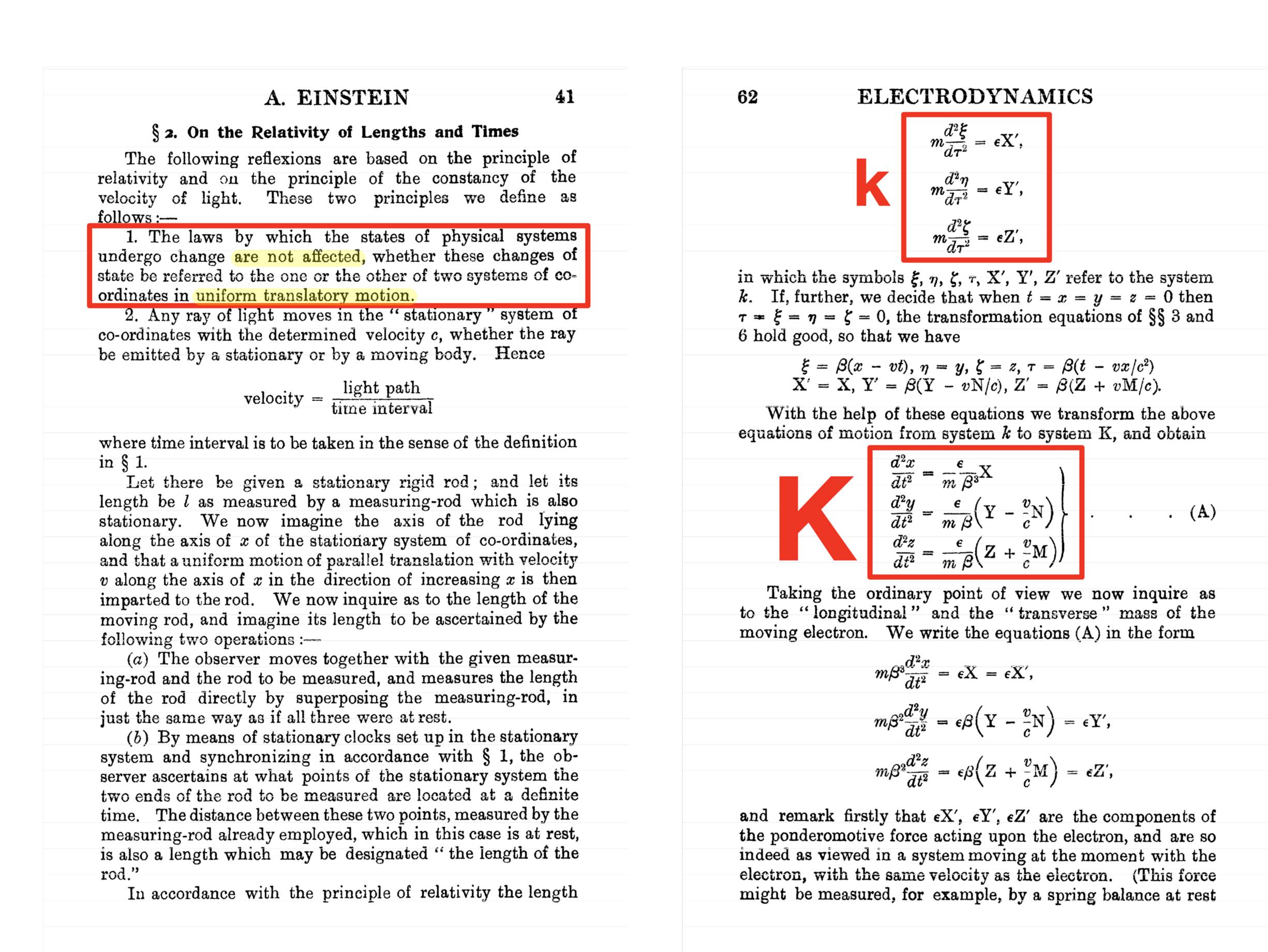
FIGURE \(13.\) Page 41 of ref.\(^{3}\), clearly postulating that uniform translatory motion is akin to rest. Page 62 of the same paper\(^{3}\) demonstrates a direct brazen violation of that postulate.
Yet, in brazen violation of that postulate, as seen at once on page 62, shown back to back with page 41 in this same FIGURE 13, the set of equations, referred to the one of the two coordinate systems in uniform translatory motion, system K, differs from the second set of equations, referred to the other of these two coordinate systems in uniform translatory motion, coordinate system kthe former contains velocity \(v\) (explicitly and implicitly through \(\beta = \frac{1}{\sqrt{1 - \frac{v^2}{c^2}}}\)), while the latter does not contain velocity \(v\). This difference indicates that the physical law has been affected, in direct contradiction with the just cited first postulate, also known as the principle of relativity, when Lorentz transformations are applied for the referring of this physical law to coordinate system K.
Although cited explicitly above, it is instructive to repeat what the postulate demandsthe first postulate forbids such affecting of any physical law, including the physical law at hand.
One may also observe the violation of the principle of relativity (violation of the first postulate), leading to the following absurd conclusion:
In
\(\S10\) of ref.\(^{3}\), shown here as FIGURE
14, containing both pages 61 and the already discussed page 62,
it is at once seen that the first equation set and the fourth equation
set therein refer to one and the same electron, in one and the same
coordinate system K, at one and the same time. However, these two
equation sets are obviously differentthe fourth set of equations
contains, among other differences, velocity \(v\), while the first
equation set does not contain velocity \(v\). This means that the
theory of relativity derives that one and the same body, in one
and the same coordinate system, obeys two different laws of motion
at the same time. This is a catastrophic nonsense, which is
demonstrated in this very simple way, mandating the immediate removal
from science of the theory of relativity.
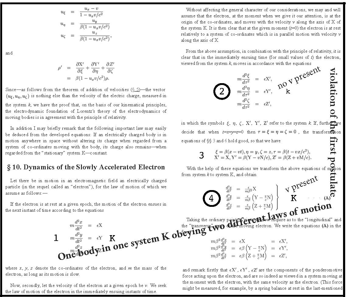
FIGURE \(14.\) Pages 62 and 63 of the original paper\(^{3}\) (translated in English) with my remarks [VCN] for prompt comprehension of the catastrophic problem invalidating at once the theory. The theory of relativity leads to the senseless conclusion that one body in one system K obeys two different laws of motion at the same timeobvious absurdity.
Although the catastrophic problem with relativity, disqualifying it altogether as having anything to do with science, is seen at once from FIGURE 14, those who are interested in more details may find them in my previous books Relativity is the Mother of All Fake News, The Pathology of Relativity and Some Notes on the General Theory of Science and No Great Reset, and especially in their ADDENDA.
The only use physics may have for said theory is to use it as a categorical proof that Lorentz transformations are non-physical and as a prop to demonstrate how physics must not be done. Therefore, everything having anything to do with these transformations must be removed from physics, and, as said, must be devoid of public funding, the way astrology and palm reading are. Remove the non-physical Lorentz transformations and all progeny such as cosmology, string theories, various projects having to do with gravity waves, Higgs boson, particle physics, high energy physics, lose any scientific basis, and therefore have no place in physics, especially funding with public funds. Thus, it should go without saying that, because anything stemming from the Lorentz transformations has no roots in reality, let alone, defying basic logic, as does the theory of relativity, any claim for experimental confirmation of the theory of relativity, and any claim connected in any way shape or form with the Lorentz transformations, is out of the question and is an outright fraud. The fatal flaws, discussed above, require immediate dissemination and action to correct the calamitous fundamental errors in current mainstream physics. These errors have been the direct cause for the crisis in physics, a crisis which has been escalating for over a century, overflowing into society at large, causing its observable demise.
False claim for deriving of \(E = mc^2\) in paper\(^{3}\)
Not only in view of the great interest the mass-energy relation \(E = mc^2\) invokes, but also, as will be seen later, because it has a direct connection with classical physics, in particular, with classical mechanics, we need to specially spell out explicitly, that the theory of relativity\(^{3}\) cannot have anything whatsoever to do with the mass-energy relation \(E = mc^2\), despite the vigorous propaganda that it does. The theory of relativity\(^{3}\) is absurdity, and therefore it cannot derive anything whatsoever, to begin with. Neither does it deserve any discussion at all.
On top of it, even if we agree, for the sake of argument, to integrate the erroneous x-axis component \(\frac{d^2x}{d t^2} = \frac{\varepsilon}{m \beta^3} X\); that is, \(m \beta^3 \frac{d^2x}{d t^2} = \varepsilon X\), of the obviously absurd eq.(A), containing the integral \( m \int_0^v \beta^3 vdv \), in \(\S10\) of ref.\(^{3}\), we will get \begin{equation*} \int{\varepsilon X dx} = \int{\beta^3 m \frac{d^2x}{d t^2} dx } \end{equation*} \begin{equation*} \int{\varepsilon X dx} = \int{\beta^3 m \frac{d v}{d t} dx} \end{equation*} \begin{equation*} \int{\varepsilon X dx} = \int{\beta^3 m \frac{d x}{d t}dv} \end{equation*} \begin{equation*} \int{\varepsilon X dx} = \int{\beta^3 m v dv}, \end{equation*}
which is the integral seen on page 63 (§\(10\)) of ref.\(^{3}\): \begin{equation}\label{confusedintegral} W = m\int_0^v{\beta^3 v dv}. \end{equation}
At this moment of the derivation, we notice something very important, which the author of ref.\(^{3}\) has deceptively confused.
Quite notably, the velocity \(v\) seen in eq.(\ref{confusedintegral}) is not the same velocity seen in the expression for the coefficient \( \beta^3 = \left( \frac{1}{\sqrt{1 - \frac{\enclose{circle}[mathcolor="red"]{\color{black}{v}}^2}{c^2}}} \right)^3\). The first derivative of velocity in \(\varepsilon X = \beta^3 m \frac{d^2x}{d t^2} = \beta^3 m \frac{d v}{d t}\) refers to the increasing velocity with respect to a given coordinate system under the action of a constant force (of course, a constant force applied at a given moment \(t\)). In contrast, the velocity \(\enclose{circle}[mathcolor="red"]{\color{black}{v}}\) in \(\beta^3 = \left( \frac{1}{\sqrt{1 - \frac{\enclose{circle}[mathcolor="red"]{\color{black}{v}}^2}{c^2}}} \right)^3\) refers to the constant velocity which the studied inertial coordinate system has with respect to another inertial coordinate system. These are two completely different velocities, absolutely not associated with each other. Notice, for example, that when no constant force is acting on the uniformly translatorily moving body at constant velocity \(\enclose{circle}[mathcolor="red"]{\color{black}{v}}\), there will be no velocity in the expression \(\varepsilon X = \beta^3 m \frac{d^2x}{d t^2} = \beta^3 m \frac{d v}{d t}\), containing the first derivative of \(v\). There, simply, will be no force at all in that expression. In fact there will be no such expression, to adorn the integral.
Therefore, for the observed systems K and k, coefficient \(\beta\) is a constant. Consequently, it can be factored out of the integral \begin{equation*} W = m \beta^3 \int_0^v{ v dv} \end{equation*} \begin{equation*} W = m \beta^3 \int_0^v{ \frac{1}{2} dv^2} \end{equation*} \begin{equation*} W = \frac{m \beta^3}{2} \int_0^v{ dv^2} \end{equation*} \begin{equation*} W = \frac{m \beta^3}{2} v^2 \Big|_0^v \end{equation*} \begin{equation} \bbox[5px, border: 2px dotted grey]{W = \beta^3 \frac{m v^2}{2}}, \end{equation}
obtaining an expression, which is only a wrong formula for the kinetic energy in K and is not at all \begin{equation} \bbox[5px, border: 2px dotted grey]{W = m c^2 \left\{ \frac{1}{ \sqrt{1 - \frac{v^2}{c^2}} } - 1 \right\}}, \end{equation} or \begin{equation} \bbox[5px, border: 2px dotted grey]{W = m c^2 \left\{ \beta - 1 \right\}}, \end{equation}
as claimed by the theory\(^{3}\). Therefore, \(E = mc^2\) cannot be derived even formally, even if we forget, for the sake of argument, the theory of relativity, and attempt to derive \(E = mc^2\) only from the Lorentz transformations, because, as just demonstrated, even this formal play with formulae, is incorrect \begin{equation} W = \int{\varepsilon X dx} = m\int_0^v{\beta^3 v dv} \ne m c^2 \left\{ \frac{1}{ \sqrt{1 - \frac{v^2}{c^2}}} - 1\right\}. \end{equation}
Thus, not only can the theory of relativity not derive anything whatsoever, but even when trying to use the Lorentz transformations alone, as non-physical as they are, all that is derived is a wrong formula for the kinetic energy in K. Even the Lorentz transformations, standalone, unassociated with the theory of relativity, cannot derive \(E = mc^2\). \(E = mc^2\) cannot be derived even formally in the specified non-classical way. Further in this book we will demonstrate the classical derivation of \(E = mc^2\), a relationship inherent in classical physics. We must also emphasize that the above exercise was completely unnecessary, and was given just for fun, as an entertaining pastime for some who may be curious, because, prior to even considering that derivation, that so-called theory of relativity, has already catastrophically collapsed on the very pages of its own 1905 paper\(^{3}\), the paper where it was first put forthrecall, the theory of relativity senselessly derives that one body in one system obeys two different laws of motion at the same time. This is an absurdity which invalidates the theory of relativity for any further consideration. The theory of relativity cannot be a part of any scientific discourse whatsoever, least of all derive anything or be the subject of any experimental testing. It is a complete, flagrant dead-end.
Another paper with a false claim for deriving of \(E = mc^2\), also a part of the fake annus mirabilis
In addition to the inability of ref.\(^{3}\) to derive \(E = mc^2\), because, aside from other problems in the derivation in ref.\(^{3}\), the theory in ref.\(^{3}\) itself is invalid, this additional so-called annus mirabilis paper, compounds the fact that the theory of relativity cannot derive \(E = mc^2\). There is no need to even analyze ref.\(^{27}\) at all, because it draws its conclusions from the equation \begin{equation} \ell^{*} = \ell \frac{1 - \frac{v}{c} cos\phi}{\sqrt{1 - \frac{\text{v}^2}{c^2}}}, \end{equation}
which is derived using the non-physical Lorentz transformations. As seen above, no physically valid relationship can be derived from a relationship which has no physical meaning, such as the Lorentz transformations. What was said so far should be enough to conclude that any further attempt to portray that the theory of relativity could derive \(E = mc^2\) must be rejected most decisively.
Dimensional analysis of Amperes law \(\nabla \times \textbf{H} = \mu_0 \textbf{J} + \varepsilon_0 \mu_0 \frac {\partial \textbf{E}} {\partial t}\), leading to to the understanding that Amperes law is an expression of \(E = mc^2\)
Later in this book we will spend time, demonstrating that \(E = mc^2\) is intrinsically part of classical physics. As heads-up, we will now demonstrate that \(E = mc^2\) in inherent in classical physics using as an example Amperes law. Amperes law \begin{equation}\label{Ampereslaw} \nabla \times \textbf{B} = \mu_0 \textbf{J} + \varepsilon_0 \mu_0 \frac {\partial \textbf{E}} {\partial t}, \end{equation}
considering that \(\varepsilon_0 \mu_0 c^2 = 1\), can be written also as \begin{equation}\label{Ampereslawconsideringemc2equals1} c^2 (\nabla \times \textbf{B}) = \frac{1}{\varepsilon_0} \textbf{J} + \frac {\partial \textbf{E}} {\partial t}, \end{equation}
where
\(\textbf{B}\) is the magnetic field \(\left[ \frac{kg}{C \
s}\right]\)
\(\textbf{E}\) is the electric field \(\left[ \frac{V}{m} \right]\)
\(\textbf{J}\) is the current density \(\left[ \frac{A}{m^2}\right]\)
\(\mu_0\) is the permeability of free space \(\left[ \frac{T \ m}{A}
\right]\)
\(\varepsilon_0\) is the permittivity of free space \(\left[
\frac{C}{N \ m} \right]\)
\(\nabla = \frac{\partial}{\partial x}\textbf{i} +
\frac{\partial}{\partial y}\textbf{j} + \frac{\partial}{\partial
z}\textbf{k}\) \(\left[ \frac{1}{m} \right]\), where \(\textbf{i}\),
\(\textbf{j}\), and \(\textbf{k}\) are the unit vectors
\(C\), \(m\), \(V\), \(kg\), \(A\), \(T\) and \(N\) being, respectively, Coulomb, meter, Volt, kilogram, Ampere, Tesla and Newton. The above dimensions of the SI units participating in the Ampere law, are standard and can be found in the Handbooks of Chemistry and Physics, for example.
It will now be shown through dimensional analysis that Amperes law is in fact a classical expression of the mass-energy relation \(E = mc^2\), a relation which the theory of relativity is unable to derive, despite the vigorous propaganda for over a century that it does.
Amperes law, eq.(\ref{Ampereslawconsideringemc2equals1}) has the following dimensions \begin{equation}\label{dimensionsofamperesequation} c^2 \left[ \frac{1}{m}\right] \times \left[ \frac{kg}{C \ s}\right] = \left[ \frac{N \ m^2}{C^2}\right] \times \left[ \frac{C}{s \ m^2}\right] + \left[ \frac{V}{m \ s}\right]. \end{equation}
The dimensions on the two sides of eq.(\ref{dimensionsofamperesequation}) must be the same. Besides, the dimensions of the two terms on the right side of the equality must also be the same. Lets check it out. The first term on the right side of eq.(\ref{dimensionsofamperesequation}) is \(\left[ \frac{N \ \require{cancel} \bcancel{m^2}}{C^{\require{cancel} \bcancel{2}}}\right] \times \left[ \frac{\require{cancel} \bcancel{C}}{s \ {\require{cancel} \bcancel{m^2}}}\right] = \bbox[5px, border: 2px solid grey]{\frac{N}{C \ s}}\), while, because \(\left[ \frac{V}{m \ s}\right] = \left[ \frac{J}{C \ m \ s}\right] = \left[ \frac{J}{C \ m \ s}\right] = \left[ \frac{N \ \require{cancel} \bcancel{m}}{C \ \require{cancel} \bcancel{m} \ s}\right]\), the second term on the right side of eq.(\ref{dimensionsofamperesequation}) is also \(\bbox[5px, border: 2px solid grey]{\frac{N}{C \ s}}\). Therefore, indeed, the two terms on the right side of eq.(\ref{dimensionsofamperesequation}) have the same dimension, and on the right side, we can work only with \(\bbox[5px, border: 2px solid grey]{ \frac{N}{C \ s}}\) and we have from eq.(\ref{dimensionsofamperesequation}) \begin{equation}\label{truncatedontheright} c^2 \left[ \frac{1}{m}\right] \times \left[ \frac{kg}{C \ s}\right] = \frac{N}{C \ s}, \end{equation}
We can now reorder eq.(\ref{truncatedontheright}), leaving \([kg] \ c^2\) on the left side of the equality \begin{equation}\label{reorderedampere} [kg] \ c^2 = \left[ \frac{m \ N \ C \ s}{C \ s} \right]. \end{equation}
Further, separately, we will observe that \(V\) has the dimensions \(V = \left[ \frac{kg \ m^2}{s^3 \ A} \right] = \left[ \frac{kg \ m^2}{s^2 \ \require{cancel} \bcancel{s} \frac{C}{\require{cancel} \bcancel{s}}} \right] = \left[ \frac{J}{C} \right] = \left[ \frac{N \ m}{C} \right]\). We will replace the last result in the right side of eq.(\ref{reorderedampere}) \begin{equation*} [kg] \ c^2 = \left[ \frac{m \ N \ C \ s}{C \ s} \right] = \left[ \frac{V \ C \ s}{\ s} \right] = \end{equation*} \begin{equation} \left[ V \ A \ s \right] = \left[ \frac{J}{\require{cancel} \bcancel{s}} \require{cancel} \bcancel{s} \right] = [J]. \end{equation}
or \begin{equation} \underbrace{[kg \ c^2]}_\text{\(mc^2\)} = \underbrace{[J]}_\text{E}, \end{equation}
expressing the dimensions of \begin{equation} \boxed{E = mc^2.} \end{equation}
The above was another demonstration that classical physics has unexplored depth, which cannot be substituted by bombastic claims for the existence of some new, hitherto unknown quantum world. Later in this book it will be further demonstrated, through analysis of the expanded Newtons second law, that \(E = mc^2\) is inherently present in classical mechanics (cf. here).
Flawed thermodynamic claim for photoelectric effect\(^{4}\)
Paper\(^{4}\)
presents another unsuccessful attempt at doing science, part of the
set of four papers which belong to the so-called annus mirabilis
quartet. The goal of the paper is to make the reader believe that the
continuous electromagnetic waves have also particle properties, by
seeking analogy of expected laws which would appear to govern these
waves with the laws of thermodynamics. The ruminations in the paper
are based on flawed conclusions from reordering Wiens law and that is
the connection with the blackbody radiation if one looks for such
connection. Paper\(^{4}\) has little to do
with Plancks law, which is justified, because the discussion is for
high values of \(\frac{\nu}{T}\), where Plancks and Wiens laws
practically coincide.
Thermodynamics backgrounda refresher that thermodynamics standardly derives \(S - S_0 = R \ \ln \frac{v}{v_0}\)
In order to dig comfortably and with adequate conviction into the sought for analogy, which would give the author\(^{4}\) the liberty to claim the unjustifiably celebrated unusual likeness of electrodynamics, devoted to describing infinitely divisible, continuous systems, to thermodynamics, describing discrete systems, we firstly must be very comfortable with the known relations between thermodynamic quantities. The hindrance, preventing such comfort, is that these (thermodynamic) relations may not always be that obvious. For example, it is not immediately obvious what the connection is between the change of entropy of an ideal gas, as a result of the change of volume. However, it is very important for the purposes of this topic, to know this relationship and its thermodynamic origin, because it is a relationship from thermodynamics, which the author\(^{4}\) utilizes to claim that its reproduction, when using quantities of electrodynamics, is a proof that electromagnetic fields which electrodynamics describes, behave just like ideal gases, as if these electromagnetic fields are consisting of discrete particles, rather than being described by continuous functions, as was the common view at the time.
Therefore, when discussing the theoretical description of photoelectricity, put forth by the author\(^{4}\) in 1905, this first section serves to refresh the memory regarding the pivotal goal of ref.\(^{4}\); namely, to advocate the idea that, see, an electromagnetic field, describing continuous, infinitely divisible, systems, can have its terms (the terms of electrodynamics) harnessed to describe its systems in terms of thermodynamics, which epitomizes discontinuitythink, for example, of gases, which comprise no further divisible entities than the atoms or molecules they consist of.
In concrete terms, the goal of ref.\(^{4}\) is to demonstrate that the thermodynamic relationship \(S - S_0 = R \ \ln \ \frac{v}{v_0}\), can be recovered in the form of \(S - S_0 = \frac{E}{\beta \nu} \ \ln \ \frac{v}{v_0}\), expressed in electrodynamics terms. This is supposed to prove that continuous electrodynamics obeys the same laws as the discontinuous thermodynamics. We, probably should say it upfront even at this beginning stageunfortunately, paper\(^{4}\) does not achieve that goal. This means that the celebrated seemingly unusual, some even portraying it as astonishing, wave-particle duality of light, has no theoretical basis. The discrete character of light has a standard explanation, founded in the works of C. I. Noninski, in the usual concepts of classical physics, observing the energy interactions amongst parts of a system in terms of exchanging energy (heat). This straightforward classical explanation we will deal with later in this book. Now we will observe in detail what exactly the confusion in paper\(^{4}\) consists of.
In order to understand the confusion in question, we first need to resort to a brief recollection about exactly what thermodynamics derives for the change of entropy when changing the volume of the system. This is important to know, because what the whole ref.\(^{4}\) is trying to convince us, is that, if we manage to find a way to express entropy in terms of electrodynamic quantities, more specifically, the change of that electrodynamic entropy when the volume is changed, and then manage to establish that the change in question has exactly the same form as the thermodynamic change of entropy as a result of changing the volume of the thermodynamic system, then we would have proved the claim that continuous electrodynamics has the properties of finitely divisible thermodynamics. In other words, what is intended to be proved, is that the electromagnetic waves, thought of as being continuous, infinitely divisible, behave, in fact, the way thermodynamic systems behave, consisting of finite no further divisible particles. Unfortunately, it will be shown, however, that it is not sopaper\(^{4}\) does not prove that there is such analogy, certifying that continuous electromagnetic waves behave as a discontinuous bunch of particles.
Now, as was said, we need the thermodynamic connection between change of entropy \(S\) and change of volume \(v\), and, as was also said, it is not something obvious. Thus, although it is a standard derivation in the courses of physical chemistry, we will present it here, just to make sure that we know for certain when discussing the problem at hand, that such connection has a firm thermodynamic basis.
We will start the derivation from the expression of the so-called Helmholtz energy, or isothermal-isochoric potential (a quantity valid for constant temperature (isothermal) \(T\), and constant volume (isochoric) \(V\)), usually denoted by \(F\). We will consider only reversible processes, and volume \(V\) will be treated as an extensive parameter, not referred to unit mass or a mole (as specific volume \(v\) is). Reverting the extensive parameters into intensive quantities will be done seamlessly at the end of the derivation. Thus, the Helmholtz potential is \begin{equation*} F = U - TS, \end{equation*}
where \(U\) is the internal energy and \(T\) is the absolute temperature (in this derivation we choose to use \(T\) as the notation of temperature, common nowadays, rather than the old-fashioned \(\theta\)). Then, \begin{equation*} dF = dU - TdS - SdT. \end{equation*}
According to the first law of thermodynamics, \(dU = \delta q + \delta w_{volume \ work}\), where \(\delta q\) is a small absolute amount \(\delta\) of the quantity itself (not a differential; that is, an operation indicating the main part of the change of a function of an independent variable, when that independent variable undergoes infinitesimal changesee more on varying a quantity in footnote\(^{66}\)) of the concrete extensive, non-state variable. The quantity reversible \(\delta w_{volume \ work}\) is a small change of the reversible work of expansion (cf. the footnote\(^{67}\) for some more on the first law of thermodynamics). Then, \begin{equation*} dF = \delta q + \delta w_{volume \ work} - TdS - SdT, \end{equation*}
which, because \(\delta w_{volume \ work} =-PdV\) (notice the minus sign, which compensates the minus sign of \(dV\) when work is done on the system, increasing its internal energy through decreasing (negatively increasing) the volume) and the definition of entropy \(dS = \frac{\delta q}{T}\) or \(\delta q = TdS\), is also \begin{equation*} dF = \require{cancel} \bcancel{TdS} - P dV \require{cancel} \bcancel{- TdS} - SdT = -P dV - SdT. \end{equation*}
Now, what is interesting about this \(dF = -P dV - SdT\) expression, is that it comprises a function \(F(V,T)\) of two variables; namely, \(V\) and \(T\), which allows us to write its full differential (recall the similar situation here) \begin{equation*} dF = \left( \frac{\partial F}{\partial V} \right)_T dV+ \left( \frac{\partial F}{\partial T} \right)_V dT. \end{equation*}
It is seen, when comparing the obtained two equations for \(dF\); namely, when comparing \(dF = -P dV - SdT\) and \(dF = \underbrace{\left( \frac{\partial F}{\partial V} \right)_T}_\text{-P} dV + \underbrace{\left( \frac{\partial F}{\partial T} \right)_V}_\text{-S} dT\), that \begin{equation*} \left( \frac{\partial F}{\partial V} \right)_T = -P \end{equation*}
and \begin{equation*} \left( \frac{\partial F}{\partial T} \right)_V = -S. \end{equation*}
Also, because \(F(V,T)\) is a state function, using the symmetry of the second derivative of a continuous function, we have \(\frac{\partial^2 F(V,T)}{\partial V \partial T} = \frac{\partial^2 F(V,T)}{\partial T \partial V}\), where, having also in mind the already said, that when comparing the obtained two equations for \(dF\); namely, when comparing \(dF = -P dV - SdT\) and \(dF = \left( \frac{\partial F}{\partial V} \right)_T dV + \left( \frac{\partial F}{\partial T} \right)_V dT\), that \begin{equation*} \frac{\partial^2 F(V,T)}{\partial T \partial V} = \left( \frac{\partial}{\partial T} \left( \frac{\partial F}{\partial V} \right) \right)_V = \left( \frac{\partial (-P)}{\partial T} \right)_V \end{equation*}
and \begin{equation*} \frac{\partial^2 F(V,T)}{\partial V \partial T} = \left( \frac{\partial}{\partial V} \left( \frac{\partial F}{\partial T} \right) \right)_T = \left( \frac{\partial (- S)}{\partial V} \right)_T. \end{equation*}
So, finally, we get the result we need (which, again, demonstrates that F(\(V\),T) is a state function) \begin{equation*} \left( \frac{\partial S}{\partial V} \right)_T = \left( \frac{\partial P}{\partial T} \right)_V, \end{equation*}
which can be rearranged, and, being in the realm of thermodynamics\(^{68}\), have the ideal gas law involved, the latter reading \(P = \frac{RT}{V}\) for \(1\) mole, \begin{equation*} dS_T = \left( \frac{\partial P}{\partial T} \right)_V dV = \frac{\partial }{\partial T} \left( \frac{RT}{V} \right)_V dV = \frac{R}{V} dV, \end{equation*}
which now may be integrated \begin{equation*} \int_{S_0}^S dS_T = R \int_{V_0}^V \frac{1}{V} dV \end{equation*} \begin{equation*} S \Bigg|_{S_0}^S = R \ \ln \ V \ \Bigg|_{V_0}^V, \end{equation*}
which, expressed as intensive parameters, gives \begin{equation}\label{thedesiredequality} \boxed{S - S_0 = R \ \ln \ \frac{v}{v_0} .} \end{equation}
Thus, here we see, rigorously thermodynamically derived, that in an isothermal process, the change of volume of an ideal gas causes change in entropy. The rigorously derived formula, shown in the box, epitomizing the discrete world of thermodynamics, is the central goal to reach in ref.\(^{4}\), aiming at proving that the infinitely divisible, continuous world of electromagnetic waves, can also derive the above formula, shown in the box, symbolizing the finitely divisible world of thermodynamics.
Unfortunately,
it can at once be seen below, in what follows, that electromagnetic
fields do not exhibit this behavior (the behavior of ideal gas) and do
not lead to an expression analogous to the expression shown above in
the box.
The flawed derivation as it is given in §\(4\) of the paper\(\S4\), invalidating the conclusions therein
Let us now follow how the attempt is carried out in paper\(^{4}\), to derive from electromagnetic relationships an equality analogous to the above-derived equality \(\boxed{S - S_0 = R \ \ln \ \frac{v}{v_0} }\), eq.(\ref{thedesiredequality}), and where exactly the problem is.
The derivation in \(\S4\) of ref.\(^{4}\) is central to the conclusions in the entire paper\(^{4}\), and its failure, as shown below, makes the theoretical backing of the wave-particle duality unsustained, as far as its thermodynamic argumentation is concerned.
It needs to be mentioned here too, that there is a legitimate derivation, contained in the C. I. Noninski paper\(^{11}\), of the particle-like behavior of electromagnetic radiation. C. I. Noninski has shown that such behavior is entirely expected according to classical physicsthe only possible way for the parts of a system to interact among themselves is through exchanging of portions of energy (heat). Thus, if one is concerned about the particle behavior of electromagnetic waves, the legitimate, physically consistent way, is along the lines of C. I. Noninskis paper\(^{11}\).
The derivation in paper\(^{4}\) is based on Wiens law, which results when the denominator \(e^{\frac{h \nu}{k T}}- 1\) in Plancks law, \(u = \frac{8 \pi \nu^2}{c^3}\frac{h \nu}{e^{\frac{h \nu}{k T}}- 1} = \frac{8 \pi h \nu^3}{c^3}\frac{1}{e^{\frac{h \nu}{k T}}- 1}\), is replaced in the denominator, for large \(\frac{\nu}{T}\), by the exponent \(e^{\frac{h \nu}{k T}}\) itself, neglecting the unity, which becomes negligibly small in comparison, under these conditions of large \(\frac{\nu}{T}\). The resultant formula is simplified even further by making the substitutions \(\frac{8 \pi h}{c^3} = \alpha\) and \(\frac{h}{k} = \beta\). Thus, the portable version of Wiens law becomes: \begin{equation}\label{firstequationinparagraph4} \rho = \alpha \nu^3 e^{-\beta \frac{\nu}{T}}. \end{equation}
After taking the logarithm of both sides \begin{equation*} \ln \rho = \ln \alpha + 3\ln\nu + (-\beta) \frac{\nu}{T}, \end{equation*}
rearranging, \begin{equation*} \beta \frac{\nu}{T} = \ln \alpha + 3\ln\nu - \ln \rho \end{equation*} \begin{equation*} \beta \frac{\nu}{T} = \ln \frac{\alpha \nu^3}{\rho} \end{equation*} \begin{equation*} \frac{1}{T} = \frac{1}{\beta \nu}\ln \frac{\alpha \nu^3}{\rho}, \end{equation*}
and reversing numerator and denominator of the quotient under the logarithm, eq.(\ref{firstequationinparagraph4}) obtains the form \begin{equation}\label{1overTexpressedfromWienslaw} \frac{1}{T} = -\frac{1}{\beta \nu}\ln \frac{\rho}{\alpha \nu^3} = const, \end{equation}
shown in \(\S4\) of paper\(^{4}\).
So far, so good. We now arrived at the second equation seen in \(\S4\) of paper\(^{4}\), which, importantly, gives what \( \frac{1}{T} \) looks like in terms of Wiens law (that is, in terms of the other parameters in the first expression in §\(4\) of paper\(^{4}\), which herewith comprise the other parameters in eq.(\ref{firstequationinparagraph4}) seen here). In the present discussion, it should also be especially emphasized here, that the expression for \(\frac{1}{T}\) in eq.(\ref{1overTexpressedfromWienslaw}) comprises a constant. It is important to pay attention to that fact, in order to keep it in mind when an integration is going to be carried out shortly. This so far was the realm of electromagnetic waves, symbolizing the world of continuity, which the author\(^{4}\) will unsuccessfully attempt to abolish by the next steps. In these follow-up steps, he will try to demonstrate that the world of continuity characterizing electrodynamics, is, in fact, only seeming, because electromagnetic waves, hitherto thought of as being only continuous entities, purportedly contain the features of thermodynamics, symbolizing the world of discontinuity, the world of particles.
Alternatively, in pursuit of his goal, failed in the end, to make a connection between the radiation theory he just exemplified by \(\frac{1}{T} = -\frac{1}{\beta \nu}\ln \frac{\rho}{\alpha \nu^3} = const\), eq.(\ref{1overTexpressedfromWienslaw}), symbolizing continuity, on the one hand, and a view based on discontinuity, on the other hand, he attempts to involve the molecular-kinetic theory of the ideal gas, which is the expression of thermodynamics; that is, the expression of particle behavior. This goal the author\(^{4}\) tries to accomplish by using the expression for \(\frac{1}{T}\); namely \(\frac{1}{T} = \frac{\partial \varphi}{\partial \rho}\), he derived thermodynamically in \(\S3\). In fact, that expression derived in \(\S3\), is an obvious expression, for whose obtainment there is no need to use variational calculus, especially if one is careful not to commit the logical fallacy petitio principii, by assuming that there is entropya thermodynamic notionin electromagnetism; that is, when the goal is exactly to prove that electromagnetism can be described by the notions of ... thermodynamics. That is, if one does mind not to commit the logical fallacy petitio principii by having the answer contained in the question. This logical fallacy is also known as circular argument or begging the question. Indeed, \(\frac{\partial \varphi}{\partial \rho}\) can be \(\frac{1}{T}\) only if \(\varphi\) is equal to \(\frac{\rho}{T} \); that is, only if \(\varphi \) is itself entropy per unit volume, corresponding to a given frequency \(\nu\). More detailed, the true equation reads \(\frac{\partial \varphi}{\partial \rho} = \frac{\partial \frac{q}{vT}}{\partial \frac{q}{v}} = \frac{ \require{cancel} \bcancel{\frac{1}{v}}\partial \frac{q}{T} }{ \require{cancel} \bcancel{\frac{1}{v}}\partial q } = \frac{1}{T}\), where \(q\) is exchanging energy (heat).
As a matter of fact, only due to this committing of petitio principii, the paper at hand must be rejected, as being a paper applying non-scientific reasoning. We will show further an even graver reason for the invalidity of the derivation in ref.\(^{4}\)
This second step (namely, the use of \(\frac{1}{T} = \frac{\partial \varphi}{\partial \rho}\)), allows the author\(^{4}\) to substitute the quotient \(\frac{1}{T}\) in electromagnetically derived \(\frac{1}{T} = -\frac{1}{\beta \nu}\ln \frac{\rho}{\alpha \nu^3} = const\), eq.(\ref{1overTexpressedfromWienslaw}), by the expression \(\frac{\partial \varphi}{\partial \rho}\) for this same \(\frac{1}{T}\) from thermodynamics, thus, getting the following hybrid equation \begin{equation}\label{oneovertintwoways} \frac{\partial \varphi}{\partial \rho} = -\frac{1}{\beta \nu}\ln \frac{\rho}{\alpha \nu^3} = const, \end{equation} instead of the purely electromagnetic eq.(\ref{1overTexpressedfromWienslaw}), \(\frac{1}{T} = -\frac{1}{\beta \nu}\ln \frac{\rho}{\alpha \nu^3} = const\), already obtained above.
As a last step, the needed expression for entropy \(d\varphi\) but expressed through electromagnetism, is obtained after rearrangement of eq.(\ref{oneovertintwoways}): \begin{equation}\label{dphi} d \varphi = -\frac{1}{\beta \nu}\ln \frac{\rho}{\alpha \nu^3} d \rho = const . d\rho. \end{equation}
Then, the author\(^{4}\) erroneously considers the constant, having the form of \(-\frac{1}{\beta \nu}\ln \frac{\rho}{\alpha \nu^3}\), as not a constant, but as a function of \(\rho\). This error allows him to use the standard fact from the table of integrals that \(\int a \ \ln b x \ dx = a x (\ln b x - 1)\) (for reading convenience, consider, in the just shown formula, the substitutions \(a = -\frac{1}{\beta \nu}\), \(b = \frac{1}{\alpha \nu^3}\) and \(x = \rho\)), and have both sides of equation (\ref{dphi}) integrated. In carrying out this integration, the author\(^{4}\) obtains the following incorrect result from the integration \begin{equation}\label{aformofphifunction} \bbox[5px, border: 2px solid grey]{ \varphi = -\frac{\rho}{\beta \nu} \left\{ \ln \frac{\rho}{\alpha \nu^3} - 1 \right\}}. \end{equation}
For a brief illustration of the essence of the error one may consider the following footnote\(^{69}\).
As an aside, accidentally, it is methodologically proper to correct the error anyway, even if this formal error would not affect the final conclusion, which will be negative anyway (the final outcome will be even worse, if the incorrect eq.(\ref{aformofphifunction}) would be used, because that outcome would have two additional terms \(\frac{v\rho}{\beta \nu}\) and \(\frac{v_0\rho}{\beta \nu}\), which cannot be canceled). Thus, it may be noted that the correct expression, after correct integration, honoring the fact that the entire expression \(-\frac{1}{\beta \nu} \ln \frac{\rho}{\alpha \nu^3}\) is a constant, is (for a frequency interval \(\nu\), \(\nu + d\nu\)) \begin{equation}\label{correctderivationofS} v \varphi d\nu = S = -\frac{v\rho}{\beta \nu}\ln \frac{\rho}{\alpha \nu^3 d\nu} \end{equation}
(cf. footnote\(^{70}\) for the correct solution of the integral).
Now, even if we accept that eq.(\ref{correctderivationofS}), or even if we accept that the result of the incorrect integration, eq.(\ref{aformofphifunction}), comprises a correctly derived formula for entropy \(S\), both of those expressions for the entropy \(S\) do not lead to the desired form of the \(S - S_0\) difference, supposed to resemble the thermodynamically derived \(S - S_0 = R \ln \frac{v}{v_0}\), because the entropy corresponding to a different volume \(v_0\), which must be subtracted from \(v \varphi d\nu = S = -\frac{v\rho}{\beta \nu}\ln \frac{\rho}{\alpha \nu^3 d\nu}\), eq.(\ref{correctderivationofS}) (represented also as \(S = -\frac{v\rho}{\beta \nu}\ln \frac{v\rho}{v\alpha \nu^3 d\nu}\), obtained by multiplying and dividing by \(v\) the quotient under the logarithm, or \(S = -\frac{E}{\beta \nu}\ln \frac{E}{v\alpha \nu^3 d\nu}\), where \(E = v \rho\)), must be \begin{equation}\label{correctsminuss0equationforv0} S_0 =\enclose{circle}[mathcolor="red"]{\color{black}{\enclose{circle}[mathcolor="red"]{\color{black}{v_0}} }}\varphi (\rho, \nu) d\nu = -\frac{\enclose{circle}[mathcolor="red"]{\color{black}{E_0 }}}{\beta \nu}\ln \frac{ \enclose{circle}[mathcolor="red"]{\color{black}{E_0 } }}{ \enclose{circle}[mathcolor="red"]{\color{black}{\enclose{circle}[mathcolor="red"]{\color{black}{v_0}}}} \alpha \nu^3 d\nu } , \end{equation}
or, if we decide to be true to the original\(^{4}\) by using only the incorrectly integrated in ref.\(^{4}\) expression for entropy, the expression for \(S_0\) must be \begin{equation}\label{sminuss0equationforv} \bbox[5px, border: 2px dotted grey]{S_0 =\enclose{circle}[mathcolor="red"]{\color{black}{\enclose{circle}[mathcolor="red"]{\color{black}{v_0}} }}\varphi (\rho, \nu) d\nu = -\frac{\enclose{circle}[mathcolor="red"]{\color{black}{E_0 }}}{\beta \nu}\left\{ \ln \frac{ \enclose{circle}[mathcolor="red"]{\color{black}{E_0 } }}{ \enclose{circle}[mathcolor="red"]{\color{black}{\enclose{circle}[mathcolor="red"]{\color{black}{v_0}}}} \alpha \nu^3 d\nu } - 1 \right\} }, \end{equation}
where \(E_0 = v_0 \rho\).
We will now use the correctly integrated expression for \(S\), eq.(\ref{correctderivationofS}), in the form of \(S = -\frac{v\rho}{\beta \nu}\ln \frac{v\rho}{v\alpha \nu^3 d\nu}\), which, didnt we say, provides, in a manner of speaking, a milder error, because in the end the result will lack the additional terms \(\frac{v\rho}{\beta \nu}\) and \(\frac{v_0\rho}{\beta \nu}\) which, additionally, cannot be canceled. Thus, by using the correctly integrated eq.(\ref{correctderivationofS}) we are doing our best to somehow help the author in obtaining a correct result, alas, in vain.
This, correct way of subtracting the entropy difference \(S - S_0\); namely, by subtracting from eq.(\ref{correctderivationofS}) the equation eq.(\ref{correctsminuss0equationforv0}) (as said, using eq.(\ref{sminuss0equationforv}) will make matters even worse), will result in \begin{equation*} S - S_0 = -\frac{v\rho}{\beta \nu}\ln \frac{v\rho}{v\alpha \nu^3 d\nu} - \left( -\frac{\enclose{circle}[mathcolor="red"]{\color{black}{v_{0} \rho}}}{\beta \nu} \left\{ \ln \frac{\enclose{circle}[mathcolor="red"]{\color{black}{v_{0}\rho}}}{\enclose{circle}[mathcolor="red"]{\color{black}{\enclose{circle}[mathcolor="red"]{\color{black}{v_0}}}} \alpha \nu^3 d\nu} \right\} \right), \end{equation*} \begin{equation*} S - S_0 = -\frac{v\rho}{\beta \nu}\ln \frac{v\rho}{v\alpha \nu^3 d\nu} + \frac{\enclose{circle}[mathcolor="red"]{\color{black}{v_{0} \rho}}}{\beta \nu} \ln \frac{\enclose{circle}[mathcolor="red"]{\color{black}{v_{0}\rho}}}{\enclose{circle}[mathcolor="red"]{\color{black}{\enclose{circle}[mathcolor="red"]{\color{black}{v_0}}}} \alpha \nu^3 d\nu} \end{equation*} \begin{equation} S - S_0 = -\frac{E}{\beta \nu}\ln \frac{E}{v\alpha \nu^3 d\nu} + \frac{\enclose{circle}[mathcolor="red"]{\color{black}{E_0}}}{\beta \nu} \ln \frac{\enclose{circle}[mathcolor="red"]{\color{black}{E_0}}}{\enclose{circle}[mathcolor="red"]{\color{black}{\enclose{circle}[mathcolor="red"]{\color{black}{v_0}}}} \alpha \nu^3 d\nu}, \end{equation}
not in the desired \begin{equation} S - S_0 = \frac{E}{\beta \nu}\ln \frac{v}{v_0}, \end{equation}
as ref.\(^{4}\) claims to derive, because the cancellations, carried out if one erroneously considers that \(v\rho = v_0\rho = E\), are impossible. We dont even need to get into further arguments\(^{28}\), as to whether or not frequency \(\nu\) changes to frequency \(\nu_0\) upon changing of volume from \(v\) to \(v_0\).
Incidentally,
even before attempting the above derivation, failed in the end, it
should be clear from the outset, that the electromagnetic waves, in
contrast to a system of particles comprising an ideal gas, have
intrinsic, undeniable properties which thermodynamically treated
particles have not, such as conditions for standing waves, depending
on the dimensions of the enclosure, different from the dependence of
the properties of the ideal gas on the dimensions of the vessel
containing them.
A simple example demonstrating the essence of the wrong method applied in ref.\(^{4}\)
The above wrong method of derivation, performed in ref.\(^{4}\), ridiculously foisting that two unequal quantities, \(v \rho\) and \(v_0 \rho\), are equal, and therefore can be canceled out, can be illustrated for immediate comprehension, by this simple example:
Lets have \begin{equation} y = e^x \end{equation}
and \begin{equation} Z = -my, \end{equation}
where \(m\) is a constant. Then, \(\ln y = x\), or \(\frac{\ln y}{x} = 1\) and \(-\frac{Z}{my} = 1\), therefore \(-\frac{Z}{my} = \frac{\ln y}{x}\) or \begin{equation} Z = - \frac{my}{x} \ln y, \end{equation}
which, when multiplying and dividing by \(m\) the quantity under the logarithm, becomes \begin{equation}\label{Z} Z = - \frac{my}{x} \ln \frac{my}{m}. \end{equation}
Then, for another constant \(m_0 \ne m\), we get \begin{equation}\label{Z_0} Z_0 = - \frac{m_0y}{x} \ln \frac{m_0y}{m_0}. \end{equation}
Therefore, from eq.(\ref{Z}) and eq.(\ref{Z_0}) we get \begin{equation*} Z - Z_0 = - \frac{my}{x} \ln \frac{my}{m} - \left( - \frac{m_0y}{x} \ln \frac{m_0y}{m_0} \right). \end{equation*} \begin{equation} Z - Z_0 = - \frac{my}{x} \ln \frac{my}{m} + \frac{m_0y}{x} \ln \frac{m_0y}{m_0}. \end{equation}
Now, the goal is to obtain \begin{equation} Z - Z_0 = \frac{my}{x} \ln \frac{m}{m_0}. \end{equation}
However, this can occur only if \(my = m_0y \), which is impossible, because: \begin{equation} m e^x \ne m_0 e^x. \end{equation}
This travesty of a derivation, whereby, in order to get the desired result, one assumes that the two unequal quantities \(m e^x \ne m_0 e^x\) are considered equal, is at the basis of the conclusions in paper\(^{4}\), which makes those conclusions unfounded in their entiretypaper\(^{4}\) has not proved the equivalence between the continuous, infinitely divisible, world of the electromagnetic waves and the discrete world of thermodynamics. Wave-particle duality does not follow from paper\(^{4}\). Particle-like character of electromagnetic waves can only be pondered in terms of classical physics, along the lines charted by C. I. Noninski, to be discussed later in this book, whereby the classical quanta have wave-like properties because the origin of these quanta is closely tied to waves.
Nothing more needs to be said about paper\(^{4}\), despite various other problems detected. It would be a waste of time presenting them, when the entire wave-particle idea in paper\(^{4}\) has collapsed altogether. As said, the correct wave-particle picture is first presented by C. I. Noninski; at that, naturally following from classical physics.
What
makes an indelible impression, is the fact that paper\(^{4}\)
regurgitates, for the umptieth time, the incredible travesty that two
unequal quantities are equal, as a method of carrying out a
derivation.
Systematic abominations
Counter-scientific
abominations, such as the one observed in paper\(^{4}\),
are systematic and symptomatic for that author. These abominations
have nothing to do with the subject of the concrete study but are a
staple of low-quality thinking. In fact, that travesty is so low that
it is no less than insulting to the reader. The shown determination by
the author of ref.\(^{4}\) to accept as equal
two obviously non-equal quantities, is a replica of what the same
author does in \(\S6\) of paper\(^{3}\),
where one reads after the third system of equations:
Evidently
the two systems of equations found for system k must express exactly
the same thing, since both systems of equations are equivalent to
the Maxwell-Hertz equations for system K.
However, what is really obvious is that the two systems of equations found for system k most evidently do not express the same thing, let alone, one of them is not equivalent to the Maxwell-Hertz equations for system K. On the contrary, the two systems in question are flagrantly differentone contains velocity \(v\), the other doesnt. The abomination seen here of the 1917 paper\(^{2}\) also carries out a derivation on the absurd premise that two unequal quantities are equal.
It is incredible that one should have such thinking, aggressively flawed, yet domineering, and that it should have so much impact on the world, entirely occupying its higher intellectual echelons.
On the earliest derivation of the particle-wave duality
The excuse that paper\(^{4}\) has shown some early way of connecting the properties of waves with the behavior of particles, which, even if unsustained, were later corrected, establishing firmly that light is made of photons, does not stand scrutiny. This is so, because every time someone begins presenting improved arguments about unusual wave-particle duality characterizing light, that someone can be confronted with the demonstration, shown here, that such picture cannot be sustained on thermodynamic basis. The portioned way of light behavior can be explained only on the basis of the exchanging energy (heat) mechanism of interaction, brilliantly proven by C. I. Noninski.
There may be any number of experimental studies claiming wave-particle duality. However, ref.\(^{4}\) does not derive that duality. Let alone that ref.\(^{4}\) proves that wave-particle duality has no thermodynamic basis. This is a conclusion that will stay on forever, without any expectation that future developments may overturn it, and that somehow it will be proven that electromagnetic waves obey thermodynamic relationships. The only correct derivation proving that light sources emit energy in portions is given by C. I. Noninski. At that, most importantly, C. I. Noninski proves this on the basis of classical physics, without postulating impossible conditions based on far-out ideas.
One can often hear dont show me how something doesnt work, show me how it works. It is understandable that one should strive to demonstrate positively how things work. However, such demonstration must never be at the expense of physical meaning and logic. Otherwise, one would fall into disgraceful voluntarism, which is as far from science as it gets. To say nothing of the fact that C. I. Noninskis study does show how it works.
We must never apply mathematical procedures which are at odds with the physical meaning of the formulae proposed, to say nothing about applying mathematical procedures that are themselves incorrect. Calling that absurd approach heuristic, as the author of ref.\(^{4}\) calls it, is not an excuse.
Now, after discussing the failed attempt to justify wave-particle duality, we will move on, finding ourselves dealing with yet another instance of non-scientific banter, faking a derivation of the blackbody formula.
Specific heat of solidsanother unsuccessful derivation of blackbody radiation expression ... and more
NOTE: In this part we will be using the same letter \(c\) for denoting both specific heat and speed of light. The meaning of \(c\) will be clear from the context. It appears that this uniform notation is less confusing than denoting speed of light by \(L\), as the author of ref.\(^{6}\) does.
Paper\(^{6}\) on anomalous specific heat of solids, although not part of the annus mirabilis papers, but considered as having comparable impact on solid-state physics, is another failed attempt by its author to derive what he calls the law of energy distribution of black-body radiation formulated by Planck\(^{1}\), but, as it happens, not at all derived by Planck (cf. here). The paper at hand\(^{6}\) adds another example to the disgraceful tendency, observed in the previously discussed cases, defying even basic criteria for a scientific study.
Although the problems in the paper in question begin from the very start, they deserve no analysis not only because they can be shown to be flawed on their own, but especially because they have no connection with the crucial errors detected on page 183 (the page number in the German original) of this same ref.\(^{6}\), crucial errors central to the derivation of the blackbody radiation formula in the paper at hand. Those who are curious may look at the consideration in footnote\(^{71}\), which pinpoints the problem in the initial part of ref.\(^{6}\), the part that may be ignored altogether anyway.
We will assume, for the sake of argument, that one manages to reach page 183 of ref.\(^{6}\), before the unacceptable flaws in the earlier parts of the derivation of the mentioned law make the reader deservedly abandon the analysis of ref.\(^{6}\)
The erroneous step in question is in the second chain of equalities on page 183 of ref.\(^{6}\), namely, in \begin{equation*} \frac{\int Ee^{-\frac{N}{RT}E} \omega(E) dE}{\int e^{-\frac{N}{RT}E} \omega(E) dE } = \frac{0 + A \varepsilon e^{-\frac{N}{RT}\varepsilon} + A 2\varepsilon e^{-\frac{N}{RT}2\varepsilon} ...}{A + A e^{-\frac{N}{RT}\varepsilon} + A e^{-\frac{N}{RT}2\varepsilon} + ...} \end{equation*} \begin{equation}\label{incorrectequality} = \frac{\varepsilon}{e^{\frac{N}{RT}\varepsilon} - 1}, \end{equation}
under the condition \begin{equation}\label{acondition} \int\limits_{\varepsilon}^{\varepsilon + a} \omega dE = \int\limits_{2\varepsilon}^{2\varepsilon + a} \omega dE ... = \int\limits_0^a \omega dE = A. \end{equation}
More specifically, the author has failed to recognize that while the right side of the first equality in eq.(\ref{incorrectequality}) indeed leads to \(\frac{\varepsilon}{e^{\frac{R}{NT}\varepsilon} - 1}\) (see in footnote\(^{72}\) why purely mathematically, the expression after the first equality, is equal to the expression after the second equality), that same right side does not follow from the left side of the first equality in eq.(\ref{incorrectequality})cf. ADDENDUM here.
The incorrect equality, eq.(\ref{incorrectequality}), does not make the integral quotient \(\frac{\int Ee^{-\frac{N}{RT}E} \omega(E) dE}{\int e^{-\frac{N}{RT}E} \omega(E) dE }\) connected in any way to a formula \(\frac{\epsilon}{e^{-\frac{N}{RT}\epsilon} - 1}\), resembling the exponential factor \(\frac{h \nu}{e^{\frac{h \nu}{k \theta}}- 1}\) (as that part of the formula is called in this book) in Plancks law. Recall also, that the pre-exponential factor \(\frac{8 \pi \nu^2}{c^3}\) (as we call it here) of Plancks law, is a non-controversial formula, stemming from absolute truths of physics, and is not at issue here.
Therefore, Plancks law, the combination of the pre-exponential factor and the exponential factor, cannot be considered as derived in ref.\(^{6}\)
Thus,
the suggested further substitution of \(\varepsilon\) by
\(\frac{R}{N}\beta \nu\) to obtain the mean energy of an oscillator in
Plancks law \(\frac{\frac{R}{N}\beta \nu}{e^{\frac{\beta \nu}{T} -
1}}\), where \(\beta = \frac{h}{k}\), \(h\) being the Planck constant,
\(k\) being the Boltzmann constant, and always keeping in mind that
\(\frac{R}{N} = k\), where \(R\) is the ideal (universal) gas constant
and \(N\) is the Avogadro number, is a substitution into a formula
which has not been derived. In conclusion, the statement on page 183
of the original of ref.\(^{6}\), that
Equation
(7) shows the dependence of the mean energy of Plancks resonator on
the temperature
arrives from nowhere, since eq.(7) has not been derived.
Thus, the debunking of the theoretical basis of ref.\(^{6}\) can be contained in only a short note comprising the last paragraphs.
Consequently,
there is no basis to claim that
From the above it emerges clearly in which sense the molecular-kinetic theory of heat must be modified in order to be brought into agreement with the distribution law of black-body radiation. For although one has thought before that the motion of molecules obeys the same laws that hold for the motion of bodies in our world of sense perception (in essence, we are only adding the postulate of complete reversibility), we now must assume, for ions capable of oscillating at particular frequencies which can mediate an exchange of energy between matter and radiation, that the diversity of states they can assume is less than for bodies within our experience. For we had to make the assumption that the mechanism of energy transfer is such that the energy of elementary structures can only assume the values 0, (R/N)\(\beta \nu\), 2(R/N)\(\beta \nu\), etc.
I believe that we must not content ourselves with this result. For the question arises: If the elementary structures that are to be assumed in the theory of energy exchange between radiation and matter cannot be perceived in terms of the current molecular-kinetic theory, are we then not obliged also to modify the theory for the other periodically oscillating structures considered in the molecular theory of heat? In my opinion the answer is not in doubt. If Plancks radiation theory goes to the root of the matter, then contradictions between the current molecular-kinetic theory and experience must be expected in other areas of the theory of heat as well, which can be resolved along the lines indicated. In my opinion this is actually the case, as I shall now attempt to show.
Unfortunately, from all seen so far, there are no grounds for such expectations, and the reader may as well abandon the so-called study, presented in ref.\(^{6}\) There is absolutely no need to continue the analysis of this gibberish.
We
will, however, keep going, only for the sake of argument and
enlightenment about the sorry state of affairs in science with its
false heroes, curious to see how far this non-scientific ramble could
go on.
\(c = 3Rn =5.94n\) not derived
Here is
the next stumbling block. When on page 184 of the original of ref.\(^{6}\),
preparing to introduce the correction, which the author of ref.\(^{6}\)
imagines he is making, of the molecular-kinetic theory of gasses, with
the goal to derive the formula of the blackbody radiation energy
density, that author invokes again the confused eq.(4), \(\overline{E}
= \frac{\int{E e^{-\frac{N}{RT}E}}dE}{\int{e^{-\frac{N}{RT}E}}dE} =
\frac{RT}{N}\), seen on page 182 of the original ref.\(^{6}\),
With
this assumption, by applying the molecular-kinetic theory (equation
(4)) while taking into account that three degrees of freedom of
motion must be assigned to each atom
thinking that it genuinely derives that \(\overline{E} = \frac{RT}{N}\); that is, that it genuinely produces \(\frac{\overline{E}}{T} = \frac{R}{N}\), and that, therefore, in the end, it genuinely yields \(c_v = Rn\) per degree of freedom, where \(n\) is the number of atoms in the molecule.
However, it is seen at once (cf. this paragraph in ADDENDUM), that the result from the chain of equalities \(\overline{E} = \frac{\int{E e^{-\frac{N}{RT}E}}dE}{\int{e^{-\frac{N}{RT}E}}dE} = \frac{RT}{N}\), seen on page 182 of the original ref.\(^{6}\), is incorrect.
The
correct result, provided in the
mentioned paragraph of ADDENDUM, is \(\overline{E} =
\frac{\int{E e^{-\frac{N}{RT}E}}dE}{\int{e^{-\frac{N}{RT}E}}dE} = E +
\frac{RT}{N}\). However, this result does not produce the expression
\(c = 3Rn =5.94n\), the numerical part calculated for \(1\) mole
(\(n\) is the number of atoms in the molecule) and three degrees of
freedom (using the value of \(R= 1.987 \left[ \frac{cal}{K \ mole}
\right]\)), claimed on page 185 of the original ref.\(^{6}\)
Failed specific heat of solids derivationfurther twists and turns
If we decide to put up with the above folly, we may proceed, out of curiosity, to see what further twists, on the back of the known Plancks formula, the author of ref.\(^{6}\) has in mind.
Thus, from what was done so far, we may only conclude that we have wasted our time. From this moment on, whatever derivations are proposed, they are not based on any contributions found in ref.\(^{6}\), but are based on the already well-known exponential factor (as we call it here) \(\frac{h \nu}{e^{\frac{h\nu}{kT}} - 1}\) of Plancks formula, as a given. In other words, paper\(^{7}\), if that paper were at all to be published (it shouldnt have, as the final analysis indicates), should have started right here, on page 186 of the original of ref.\(^{6}\)
More
specifically, we must note that the author of paper\(^{6}\)
has no grounds to conjecture that
Based
on the above one should note here the following: If we conceive of
the carriers of heat in solids as periodically oscillating
structures whose frequency is independent of their oscillation
energy, then according to Plancks theory of radiation we should not
expect the value of the specific heat always to be 5.94 n.
Neither Planck\(^{1}\), nor the author of paper\(^{6}\), have derived that the expression \(\frac{h \nu}{e^{\frac{h\nu}{kT}} - 1}\) is the mean energy of a single resonator. On top of it, as was seen, the author of paper\(^{6}\) did not derive \(\frac{h \nu}{e^{\frac{h\nu}{kT}} - 1} \) even formally. Least of all was the expression \(\frac{h \nu}{e^{\frac{h\nu}{kT}} - 1}\) derived based on the premise that said mean energy of the resonator is finitely divisible. Physics, let alone mathematics in paper\(^{6}\), is gone. Neither paper\(^{1}\), nor paper\(^{6}\), have any connection with physicsthe most these texts can be used for, the use of paper\(^{6}\) being none even for that purpose, is as an engineering tool, the way engineers use empirical formulae to ensure their practical goals. The most the author of ref.\(^{6}\) could do is use that expression only formally, as a curve-fitted function, to the existing experimental data regarding the specific heat of some elements, showing anomalous behavior with temperature. The reason why such curve-fitting procedure is of no scientific interest is, because it is not in a position to study the essence of the phenomena, and eventually explain it. On top of it, as is and will be seen, paper\(^{6}\) cannot fulfill even this minimal goal.
Therefore, any insinuation to the effect that scientific conclusions are to be expected from using the formula in question, is moot and must be ignored.
In what follows, we will explore whether even this curve-fitting goal is accomplished and will be established that paper\(^{6}\) cannot be used even as an instrument of curve-fitting.
We
are presented with a graph, FIGURE
15 of the experimental results for the specific heat of diamond
at different temperatures, shown in a table, FIGURE
16. The first two columns in the Table shown in FIGURE
16 are self-explanatorythe first column shows the temperature
in \([K]\), while the second column shows the corresponding
experimental values of the specific heat of diamond. The meaning of
the third column will become clear shortly, although, even knowing its
meaning, that third column will not be of much use to our analysis.
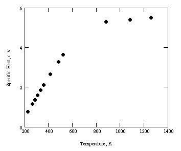
FIGURE \(15.\) Experimental data for the specific heat of diamond from ref.\(^{6}\)
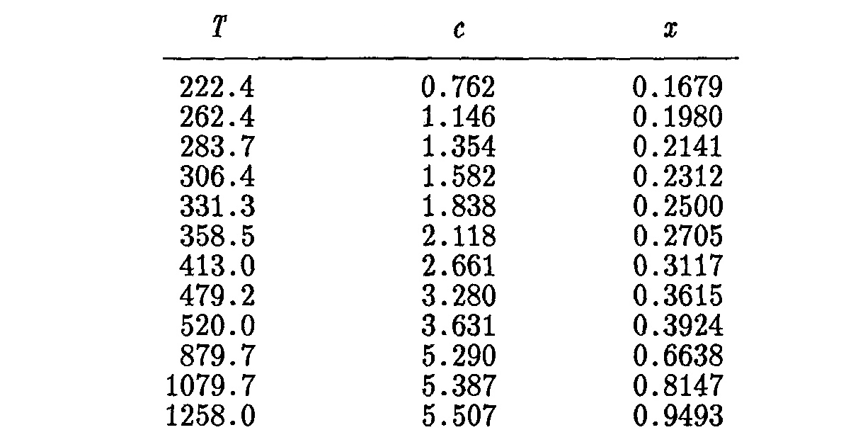
FIGURE \(16.\) Table of experimental specific heats of diamond (second column), determined for the given temperature (first column) shown on page 190 of ref.\(^{6}\). The meaning of the inconsequential numbers in the third column is discussed in the text.
The graph seen in FIGURE 15 displays anomalous behavior of the experimentally found values of the specific heat of diamond in the lower range of temperatures.
Now, the author\(^{6}\) advances as the main point of his study, finding a formula, which will reflect that anomalous run of the specific heat and explain it.
Everything the author of ref.\(^{6}\) does further, after the shown insurmountable hurdle, standing in the way of deriving Plancks law, is to make it appear that Plancks law, known as a mathematical construct anyway, is somehow connected to Dulong and Petits formula \(c_v = 3R\), concerning the specific heat of solids and to many compounds in the solid aggregation state\(^{6}\). The goal is giving the appearance that the \(R\) in the known Dulong and Petit law \(c = 3R\) can be corrected by using some formal modification of the expression \(\frac{h \nu}{e^{\frac{h\nu}{kT}} - 1}\), so that it can accommodate the specific heat of elements, exhibiting anomalous values of their specific heat at the lower range of temperatures, moreover, claiming that quantum effects are responsible for the anomalies of the specific heats of solids.
We need to note right away that there are elements that do not display anomalous values of specific heat, but they are unaccounted for by the empirical connection intendedthere is simply no ingrained criterion in the formula, correcting for the said anomalies, which would account for the elements exhibiting non-anomalous specific heat, and will trigger the dropping of the correction factor. In our usual manner of exploring even obviously deficient claims, in order to get to the bottom of the problem, we will explore the curve-fitting procedure, as tailored to each given element as it is, to see whether even with this deficiency it reaches the matching goal.
This attempted adjustment of the Dulong and Petit formula comprises the imagined great achievement of ref.\(^{6}\), thought to have corrected the theory concerned with the anomalous specific heats of solids. Unfortunately, ref.\(^{6}\) achieves no theoretical breakthrough because even its originator, Planck\(^{1}\), failed in his theorizing and presuming that energy of the resonator is not continuous, but is inherently grainy; that is, finitely divisible.
Moreover, ref.\(^{6}\) not only fails in a purely mathematical way to derive \(\frac{h \nu}{e^{\frac{h\nu}{kT}} - 1}\), as seen, which does not allow the author to even reach the point at which he may begin positing any physical picture whatsoever, but also, as seen below, he hardly accomplishes the most modest of all goals concerning an established experimental dependence; namely, independently finding the formula which would approximate the run of the experimental dependence.
Before
submerging ourselves into the curve-fitting steps he undertakes, we
should also note, as an aside, that the author's physical picture,
once again, is in discord with the real meaning of the physical
quantities. Thus, he has further failed to notice that the formula
\(\frac{\frac{R}{N}\beta \nu}{e^{\frac{\beta \nu}{T} - 1}}\) he uses
for his exercise, is the expression for the average energy
\(\overline{\varepsilon}\) (in Plancks notation, \(U\)) of a single
resonator, written by Planck in ref.\(^{1}\)
(not derived, as seen above). Indeed, says Planck\(^{1}\)
The
constant energy \(U\) of a single stationary vibrating resonator
accordingly is to be taken as time average, or what is the same
thing, as a simultaneous average of the energies of a large number
\(N\) of identical resonators, situated in the same stationary
radiation field, and which are sufficiently separated so as not to
influence each other directly.
and is far from the Dulong and Petit formula. The expression \begin{equation}\label{theplancksexpression} \overline{\varepsilon} = \frac{h \nu}{e^{\frac{h\nu}{kT}} - 1} \end{equation}
is valid for all \(3\) degrees of freedom (if \(3\), not \(2\), as is the case, were the number of degrees of freedom of a harmonic oscillator), not for just one degree of freedom, or, as the author of ref.\(^{6}\) puts it while taking into account that three degrees of motion must be assigned to each atom due to which he places the coefficient \(3\) in the, otherwise underived to begin with, formula \(c = 3Rn\) for a gram-equivalent of substance (where \(n\) denotes the number of atoms in the molecule).
Therefore, multiplication by \(3\) of \(\overline{\varepsilon} = \frac{h \nu}{e^{\frac{h\nu}{kT}} - 1}\), eq.(\ref{theplancksexpression}), is a frivolous adjustment to give the appearance of Dulong and Petits rule.
Nevertheless, it has occurred to the author of ref.\(^{6}\), for no apparent reason, but only by analogy, because he has seen that the Dulong and Petit rule contains the number \(3\), that this same coefficient \(3\) must be put in every instance when entities serving as carriers of heat in solids resemble unfoundedly imagined periodically oscillating structures whose frequency is independent of the energy of their oscillating energy, specifically the way it is described by Planck. That is, the author proposes that every time one imagines as carriers of heat in solids such structures described by Planck, one should jump at the opportunity to slap a multiplier \(3\) as soon as an \(R\) pops-up in the formula of the mean energybecause then, that mean energy, referred to temperature, will give specific heat; at that, on the one hand, resembling Dulong and Petite rule (where \(R\) is multiplied by \(3\)), and on the other, undergoing correction for the peculiarities that the periodically oscillating structures as carriers of heat in solids, may surprise us with. As said, even if we agree with that, it does not account for the non-anomalous cases, in order for this new expression, containing correction of \(R\), to be considered a general rule, replacing the Dulong and Petit rule for all cases. As was said, we will forego this problem, for the sake of the discussion, and will carry on.
It is just curious to note that, if this new Dulong and Petit law, corrected for anomalies, had any scientific merit, while coexisting with the known Dulong and Petit law, that would resemble the coexistence of Maxwells equations and the Lorentz force, a force these equations cannot derive, although they should, if they are to be general equations of electrodynamics in a scientific sense. As was seen, even the so-called theory of relativity, which was specifically created to resolve this problem was unable to (we say as was seen because we really did see that said theory is a flagrant absurdity, therefore, unable to derive anything whatsoever). This last remark, concerning Maxwells equations, was made by the way, as an aside.
The author\(^{6}\), unfortunately, has misinterpreted eq.(\ref{theplancksexpression}), \(\overline{\varepsilon} = \frac{h \nu}{e^{\frac{h\nu}{kT}} - 1}\), considering, in error, that it refers to \(1\) degree of freedom, although the mean energy \(\overline{\varepsilon}\) (in Plancks notation, \(U\)) is clearly the mean energy of the resonator referring to all degrees of freedom. Planck even states this explicitly, as was cited. As a result, the author\(^{6}\) erroneously multiplies \(\overline{\varepsilon} = \frac{h \nu}{e^{\frac{h\nu}{kT}} - 1}\) by \(3\), thinking that in this way he would account for the \(3\) degrees of freedom, which he imagines the carriers of heat in solids are characterized by (apropos, if they were to be Planck-like periodically oscillating structures, even imagined as carriers of heat, and we should at all talk (no, we shouldnt) about their degrees of freedom, their degrees of freedom are \(2\), not \(3\), as noted above). Thus, all justifications the author\(^{6}\) makes for the appearance of this multiplier \(3\), are baselessthe number \(3\) appears due to the mere resemblance to the \(3\) in the Dulong and Petit law.
On
the other hand, independently of the failed attempt for a physical
justification of the coefficient \(3\), the advocate of paper\(^{6}\)
may venture to say, well, a correction for anomalous specific heat is
attempted in a formula \(c = 3R\), which works perfectly well in many
cases, so what is wrong with using that formula, and modify it for the
menacing cases, by introducing an appropriate correction coefficient,
to become \(c = 3(R \times a \ correcting \ coefficient)\)? This
approach works perfectly well for empirical formulae which engineers
use, wrought with adjusting coefficients for each case of fulfilling
their practical goals. Unjustified adjustments, just to have a formula
fit experimental data, is not acceptable in science. There are times
when such adjustments are used, but such ad hoc repairs do not
characterize good science, and only are applied when some practical
needs require it. Anyway, let us also overlook this problem, and see
what the further steps will surprise us with.
Formation of the missing \(R\)
Now, here is an outcome in the search for \(R\) in the Dulong-Petit formula, but an \(R\) emerging straight from Plancks construct \(\overline{\varepsilon} = \frac{h \nu}{e^{\frac{h\nu}{kT}} - 1}\).
Boltzmanns constant \(k\) is \(k = \frac{R}{N}\), where \(R\) is the universal gas law constant and \(N\) is the Avogadro number, from which one can rewrite eq.(\ref{theplancksexpression}) as \(\overline{\varepsilon} = \frac{h \nu}{e^{\frac{h\nu}{kT}} - 1} = \frac{ \frac{k}{k}h \nu}{e^{\frac{h\nu}{kT}} - 1} = \frac{ k\frac{h}{k} \nu}{e^{\frac{h\nu}{kT}} - 1} = \frac{ \frac{R}{N}\frac{h}{k} \nu}{e^{\frac{h\nu}{kT}} - 1}\) \begin{equation*}\label{explicitR} \overline{\varepsilon} = \frac{R}{N} \frac{\frac{h}{k} \nu}{e^{\frac{h\nu}{kT}} - 1} \end{equation*} \begin{equation}\label{evenmoreexplicitR} \overline{\varepsilon} = R \frac{\frac{h}{k} \nu}{Ne^{\frac{h\nu}{kT}} - 1}, \end{equation}
as the author of ref.\(^{6}\) has done, in order to have explicitly the universal gas constant \(R\) as part of the formula, serving as a hint towards the correction of the known Dulong and Petit formula \(c_{\text{v}} = 3R= 3 \times 1.987 = 5.961 \left[ \frac{cal}{K \ mole} \right]\) (in ref.\(^{6}\) \(3R = 5.94 \left[ \frac{cal}{K \ mole} \right]\)).
Now,
all that is missing in eq.(\ref{evenmoreexplicitR}), in order to have
full resemblance to Dulong and Petit formula, is the missing
coefficient \(3\). We will play along with the author of ref.\(^{6}\),
keeping in mind that we do that purely for the purposes of analogy,
without any theoretical reason to do so. This is another, this time
small, concession, provided that we already know that we are headed
towards an empirical solution, not a solution having theoretical
basis.
Corrected \(R\) multiplied by \(3\)isnt that logical?
Now, let us forget about the \(3\) degrees of freedom. Then, if expressing the mean energy \(\overline{\varepsilon}\) (as we denote \(U\) here) of one resonator, is to be considered some sort of appropriate tool for correcting \(R\), in order to account for the anomalies in specific heat when expressed by the Dulong and Petit rule, then, eq.(\ref{evenmoreexplicitR}); that is, Plancks very formula for \(U\) itself (!), would be an obvious candidate. Further, one may also agree, purely formally, for reasons of analogy, to multiply that expression, with \(R\) explicitly plucked out, by \(3\); that is, getting \(3R \frac{\frac{h}{k} \nu}{Ne^{\frac{h\nu}{kT}} - 1}\). This seems what the author of ref.\(^{6}\) should logically have explored, right at this moment, whether this would result in the correct run, given by experiment, of the anomalous specific heat curve as a function of \(T\). In other words, the author should have explored if the following rule \begin{equation}\label{DulongAndPetitwithcorrectedRfirst} c = 3R \frac{\frac{h}{k} \nu}{N\left(e^{\frac{h\nu}{kT}} - 1\right)}, \end{equation}
would have been in agreement with the experimental data for anomalous specific heat of solids, providing relief from that anomaly. Notice, we write \(c\) instead of \(c_v\), because the alleged \(c\) arrives from the expression for \(1\) resonator, while reserving \(c_v\) for \(1\) mole of resonators.
However,
as seen from FIGURE
17, whereby the alleged corrected specific heat, given by
eq.(\ref{DulongAndPetitwithcorrectedRfirst}), is plotted against
temperature, shows an entirely different shape from what the shape of
the specific heat vs. temperature curve is supposed to be, as known
from experimentreaching a plateau.
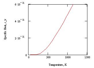
FIGURE \(17.\) Run of \(c_v\) vs. \(T\) curve with corrected \(R\) in Dulong and Petit law according to eq.(\ref{DulongAndPetitwithcorrectedRfirst}).
Therefore, treating Plancks formula \(\frac{h\nu}{e^{\frac{h\nu}{kT}} - 1} = R \frac{\frac{h}{k} \nu}{Ne^{\frac{h\nu}{kT}} - 1}\), (see eq.(\ref{evenmoreexplicitR})), as some kind of a corrected form of \(R\), having the potential to be part of some sort of a corrected form of Dulong and Petit law, in order to account for anomalous specific heat, is off the mark.
As a matter of fact, we should have known that unfavorable outcome by realizing that the expression \(\frac{\frac{h}{k} \nu}{Ne^{\frac{h\nu}{kT}} - 1}\) (the correcting factor for \(R\)), when multiplied by \(R\), becomes par excellence identical to the expression \(\frac{h\nu}{e^{\frac{h\nu}{kT}} - 1}\). The latter is nothing other than the mean energy of a resonator, and therefore, neither \(\frac{\frac{h}{k} \nu}{Ne^{\frac{h\nu}{kT}} - 1}\), nor \(3\frac{\frac{h}{k} \nu}{Ne^{\frac{h\nu}{kT}} - 1}\) can be any correction for \(R\) in the desire to use it as an alternative expression for specific heat. After all, the dimension of \(\frac{\frac{h}{k} \nu}{Ne^{\frac{h\nu}{kT}} - 1}\) is \([K]\), which multiplied by \(R\) results in energy, \(J\), not in \(\frac{J}{K}\), as the specific heat units are expected to be.
Well,
that was a failed attempt, which we should have foreseen and not
wasted time on it, but, nevertheless, it was fun doing it. After all,
is this the first instance of wasting our time, considering that all
the rest that we talked about so far, are also time-wasting instances
imposed in a major way by the mainstream? So, let us carry on and see
what the next step will offer.
How about using \(\overline{E}\) divided by \(T\)?
Or, maybe we can plot the alleged molar specific heat, obtained by multiplying the mean energy \(\overline{\varepsilon}\), eq.(\ref{evenmoreexplicitR}), by the Avogadros number \(N\) to get the mean energy \(\overline{E}\) per \(1\) mole of resonators, and then divide the result by temperature \(T\), the way the alleged mean energy for \(1\) mole, \(\overline{E}\), wrongly written as eq.(4) on page 182 of ref.\(^{6}\), was divided by \(T\), to obtain on page 185 of ref.\(^{6}\) the formula \(c = 3Rn\) (additionally frivolously, just for the sake of analogy, multiplied by \(3\)recall that detail, discussed here \begin{equation}\label{DulongAndPetitwithcorrectedRoverT} c = 3R \frac{\frac{h}{k} \nu}{TN\left(e^{\frac{h\nu}{kT}} - 1\right)}, \end{equation}
in this way, by dividing by \(T\), we resolve the above dimensional problem, making the factor \(3\frac{\frac{h}{k} \nu}{TN\left(e^{\frac{h\nu}{kT}} - 1\right)}\), supposed to correct \(R\) in the Dulong and Petit formula, dimensionless, thus, turning it into a formula which should, expectedly, account for the anomalous specific heat of some solidsnotice, the dimensions of the expression \(3R \frac{\frac{h}{k} \nu}{TN\left(e^{\frac{h\nu}{kT}} - 1\right)}\) are determined only by the dimensions of \(R\).
We can even use Wolfram Alpha to plot eq.(\ref{DulongAndPetitwithcorrectedRoverT}) for the values of constants expressed in SI units and \(\nu = 8 \times 10^{14} [Hz]\) \begin{equation*} \scriptsize \verb|plot (3*6.0221367*10^(23)*((6.6260755*10^(-34))/(1.380658*10^(-23)) | \end{equation*} \begin{equation*} \scriptsize \verb|*8*10^(14))/(6.022*10^(23)x*e^((6.6260755*10^(-34)*8*10^(14))/ | \end{equation*} \begin{equation*} \scriptsize \verb|(1.380658*10^(-23)*x)) - 1)) for x = 400 to x = 1000 | \end{equation*}
where
\(x\) is temperature, seen on the x-axis, while the y-axis is the
calculated alleged \(c_v\). This plot also does not show the expected
run of the \(c_v-T\) curve, which must reach a plateau.
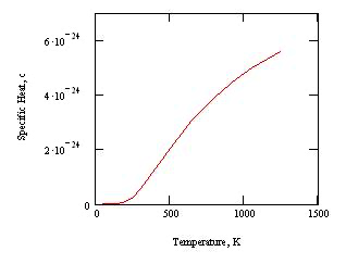
FIGURE \(18.\) Plot of eq.(\ref{DulongAndPetitwithcorrectedRoverT}).
Thus, the mere appearance of \(R\), which the author of ref.\(^{6}\) spent some effort to pluck out, in the remodeled, known Planck formula, eq.(\ref{evenmoreexplicitR}), cannot be a justification for connecting this formula to the Dulong and Petit law, and begin claiming that, now, because of Dulong and Petit, Planck should have derived for a single resonator the following \begin{equation} 3\overline{\varepsilon} = 3\frac{h \nu}{e^{\frac{h\nu}{kT}} - 1} = 3\frac{R}{N} \frac{\frac{h}{k} \nu}{e^{\frac{h\nu}{kT}} - 1}, \end{equation}
or even
\begin{equation} 3\frac{\overline{\varepsilon}}{T} = 3\frac{h
\nu}{Te^{\frac{h\nu}{kT}} - 1} = 3\frac{R}{N} \frac{\frac{h}{k}
\nu}{Te^{\frac{h\nu}{kT}} - 1}. \end{equation}
Try now with derivative of \(\overline{\varepsilon}\) over \(T\)
Further, if Plancks formula for \(\overline{\varepsilon}\) is to be used for determining specific heat by taking the first derivative of \(\overline{\varepsilon}\) over temperature \(T\), as the author of ref.\(^{6}\) has suggested, then specific heat should be determined by \(c_{v} = \frac{d \overline{\varepsilon}}{dT}\) and not by \(c_{v} = 3\frac{d \overline{\varepsilon}}{dT}\), as the author of ref.\(^{6}\) has unfoundedly done, incorrectly assuming that \(\overline{\varepsilon}\) pertains to only \(1\) degree of freedom. Then, using the real Planck formula for \(\overline{\varepsilon}\), the alleged specific heat, \(c = \frac{heat \ (energy)}{temperature}\), should be calculated as \begin{equation*} c = \frac{d}{dT} \left( \frac{h \nu}{e^{\frac{h\nu}{kT}} - 1} \right) = \frac{(h\nu)^2 e^{\frac{h\nu}{kT}} }{kT^2 \left( e^{\frac{h\nu}{kT}} - 1 \right)^2} = \end{equation*} \begin{equation} k\frac{(h\nu)^2 e^{\frac{h\nu}{kT}} }{k^2T^2 \left( e^{\frac{h\nu}{kT}} - 1 \right)^2}. \end{equation}
However, if we need to obtain the formula of the derivative in a form, such that the whole expression \(\frac{h\nu}{kT}\) be treated as the independent variable, as is done in ref.\(^{6}\)cf. the third formula from the top on page 186 of ref.\(^{6}\)we have to divide both the numerator and the denominator by \((kT)^2\) and get \begin{equation} c = \frac{d}{dT} \left( \frac{h \nu}{e^{\frac{h\nu}{kT}} - 1} \right) = k \frac{\left(\frac{h\nu}{kT}\right)^2 e^{\frac{h\nu}{kT}} }{ \left( e^{\frac{h\nu}{kT}} - 1 \right)^2}, \end{equation}
which for \(1\) mole is \begin{equation} \scriptsize c_{v} = \frac{d}{dT} \left(N \frac{h \nu}{e^{\frac{h\nu}{kT}} - 1} \right) = kN \frac{\left(\frac{h\nu}{kT}\right)^2 e^{\frac{h\nu}{kT}} }{ \left( e^{\frac{h\nu}{kT}} - 1 \right)^2} = R \frac{\left(\frac{h\nu}{kT}\right)^2 e^{\frac{h\nu}{kT}} }{ \left( e^{\frac{h\nu}{kT}} - 1 \right)^2}, \end{equation}
and if we express \(R\) as \(1.987\left[ \frac{cal}{K \ mole} \right]\), it becomes \begin{equation}\label{correctfirstderivativeoverTfromthePlankLaw} c_{v} = 1.987 \frac{\left(\frac{h\nu}{kT}\right)^2 e^{\frac{h\nu}{kT}} }{ \left( e^{\frac{h\nu}{kT}} - 1 \right)^2} = R \frac{\left(\frac{h\nu}{kT}\right)^2 e^{\frac{h\nu}{kT}} }{ \left( e^{\frac{h\nu}{kT}} - 1 \right)^2}, \end{equation}
which is \(3\) times less than the quantity shown in the third formula from the top on page 186 of ref.\(^{6}\)
It
is eq.(\ref{correctfirstderivativeoverTfromthePlankLaw}) that should
be the subject of analysis and comparison with experimental data, not
the third equation from the top, shown on page 186 of ref.\(^{6}\)
The correct comparison is presented in FIGURE
19.
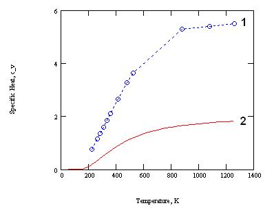
FIGURE \(19.\) Comparison of \(c_{v}\) vs. \(T\) curve obtained from first and second column of the table shown on page 190 of ref.\(^{6}\) (curve 1) with the \(c_{v}\) vs. \(T\) curve obtained from eq.(\ref{correctfirstderivativeoverTfromthePlankLaw}) (curve 2).
It is seen from the above that derivation of a formula to account for the anomalous specific heats of solids, has not been achieved. What is proposed is adjustment of formulae to fit the experimental data. It is not enough to say, well, if I perform these mathematical steps, this will lead me to coincidence with the experiment. That coincidence must be justified physically, not by just juggling with formulae. Juggling with formulae is curve fitting and there are more powerful mathematical methods to do that.
We,
however, have already agreed that for reasons of sheer analogy, we
will multiply the right side of
eq.(\ref{correctfirstderivativeoverTfromthePlankLaw}) by \(3\). In
such a case, it appears that there is almost full coincidence between
the theoretical and the experimental curvecf. FIGURE
20
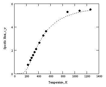
FIGURE \(20.\) Experimental data, solid dots and the curve of the expression \(5.94 \frac{\left(\frac{h\nu}{kT}\right)^2 e^{\frac{h\nu}{kT}} }{ \left( e^{\frac{h\nu}{kT}} - 1 \right)^2}\) (dashed curve) as a function of temperature \(T [K]\).
At first glance, looking at FIGURE 20, it seems that the goal of the curve-fitting exercise is accomplisheda dimensionless correcting factor \(3\frac{\left(\frac{h\nu}{kT}\right)^2 e^{\frac{h\nu}{kT}} }{ \left( e^{\frac{h\nu}{kT}} - 1\right)^2}\), multiplying the universal gas constant \(R\), expressed in paper\(^{6}\), having the units of \(\left[ \frac{cal}{K \ mole} \right]\), \(R = 1.98 \left[ \frac{cal}{K \ mole} \right]\), appears to have been found. As a reminder, as in the previous case (eq.(\ref{DulongAndPetitwithcorrectedRoverT})), the dimensions of the expression \(c = 3R\frac{\left(\frac{h\nu}{kT}\right)^2 e^{\frac{h\nu}{kT}} }{ \left( e^{\frac{h\nu}{kT}} - 1\right)^2}\) for the specific heat, are determined by the dimensions in which the ideal gas constant \(R\) is expressed.
To plot the dashed curve (the theoretical curve) in FIGURE 20 we have used the value \(\lambda = 1.1 \times 10^{-5}[m]\), as did the author of ref.\(^{6}\) (not knowing why he chose that value), which corresponds to \(\nu = \frac{c}{\lambda} = \frac{299792458}{1.1 \times 10^{-5}} = 2.72539 \times 10^{13} [Hz]\), given in ref.\(^{6}\)
All
looks well and good. However, there is a hidden problem in that
ostensible full coincidence. When inspecting all the constants taking
part in the plotted theoretical equation \(c =
3R\frac{\left(\frac{h\nu}{kT}\right)^2 e^{\frac{h\nu}{kT}} }{ \left(
e^{\frac{h\nu}{kT}} - 1\right)^2}\) (the dashed curve in FIGURE
20), we see that
Planck
constant \(h = 6.6260755 \times 10^{-34} [J \ s]\)
Boltzmann
constant \(k = 1.380648 \times 10^{-23} \left[ \frac{J}{K} \right]\)
and
the
speed of light \(c = 299792458 \left[ \frac{m}{s} \right]\), which we
use to convert \(\nu\) into \(\lambda\) by the formula \(\lambda =
\frac{c}{\nu}\)
are all
known constants; temperature \(T\) is the independent variable.
However, where did the value of the \(\nu\) come from? This is the
crucial problem, which is not at all solved in the manner proposed in
ref.\(^{6}\) for determining that missing
value of \(\lambda = \frac{c}{\nu}\), which one reads on page 189 in
the original of the paper\(^{6}\)
(translated):
Finally,
we will also apply the theory to diamond. Its infrared proper
frequency is not known, but can be calculated on the basis of the
theory described if the molecular specific heat \(c\) is known for
some temperature \(T\); the \(x\) corresponding to c can be taken
directly from the curve, and \(\lambda\) is then calculated from the
relation \(\frac{TL}{\beta \lambda} = x\) [where \(L\) denotes the
speed of light, and \(\beta = \frac{h}{\nu}\)], therefore,
\(\frac{TL}{\beta \lambda} = \frac{kT}{h \nu}\)].
This, however, is nothing else but fudging. If the value of \(\lambda = \frac{c}{\nu}\) is to be determined from the theoretical \(c_{theoretical}-\frac{kT}{h\nu}\) for a value \(c_{theoretical}\) coinciding with the \(c_{experimental}\), and then \(\nu\) is determined from that value by reordering; namely \(\nu = \frac{kT}{h c_{experimental}}\), this means that the experiment is used to justify the experiment, presenting that as if it is a theoretical result predicting the outcome of the experiment.
Look what has been donea value (frequency, respectively, wavelength) extracted from the experimental data (experimental specific heat) is used to prove coincidence of the theoretical value (of specific heat) with the experimental data (with that same value of specific heat).
Now,
it may be instructive to demonstrate how much the position in the
graph of the discussed curves depends on the chosen frequency. FIGURE
21 shows how sensitive the position of the dashed curve can be
as a result of even a slight change in the value of \(\nu\).
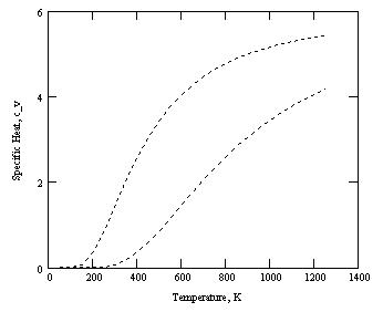
FIGURE \(21.\) Plots of \(c_v = 3R\frac{\left(\frac{h\nu}{kT}\right)^2 e^{\frac{h\nu}{kT}} }{ \left( e^{\frac{h\nu}{kT}} - 1\right)^2}\) vs. \(T\). Sensitivity wrt \(\nu\) due to mere doubling of \(\nu\)the curve on the right.
Even
more pronounced is the sensitivity with respect to the frequency value
when \(c_v = 3R\frac{\left(\frac{h\nu}{kT}\right)^2
e^{\frac{h\nu}{kT}} }{ \left( e^{\frac{h\nu}{kT}} - 1\right)^2}\) is
plotted against \(\frac{kT}{h\nu}\), the way the figure on page 186 in
ref.\(^{6}\) is plotted. We will discuss this
figure in the next section.
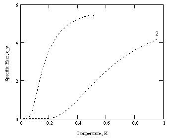
FIGURE \(22.\) \(c_v = 3R\frac{\left(\frac{h\nu}{kT}\right)^2 e^{\frac{h\nu}{kT}} }{ \left( e^{\frac{h\nu}{kT}} - 1\right)^2}\) is plotted against \(\frac{kT}{h\nu}\) for two values of \(\nu\), everything else the same. Curve 1\(\nu = 2.72 \times 10^{13} [Hz]\), curve 2\(\nu = 5.44 \times 10^{13} [Hz]\).
The
sensitivity with respect to positioning of the experimental data in
the plot, affected by the value of \(\nu\), is also illustrated in FIGURE
23, in which the experimental data for the specific heat of
diamond at various temperatures, seen in the second column of the
Table on page 190 of ref.\(^{6}\) (FIGURE
16) are plotted against \( \frac{kT}{h\nu}\) for two values of
\(\nu\)the data marked by \(\bullet\) refer to \(\nu = 2.72 \times
10^{13} [Hz]\) and these are the numbers seen in the third column of
the Table in FIGURE 16,
while the data marked by + refer to the doubled value of the
frequency; namely, to \(\nu = 5.44 \times 10^{13} [Hz]\).
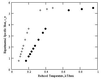
FIGURE \(23.\) Experimental data
from the specific heat of diamond, shown in the Table on page 190 of
ref.\(^{6}\) (FIGURE
16 here) plotted against \(\frac{kT}{h\nu}\) for two values of
\(\nu\), everything else the same: the data marked with solid
circles \(\bullet\) correspond to \(\nu = 2.72 \times 10^{13}
[Hz]\), while the data marked with + correspond to \(\nu = 5.44
\times 10^{13} [Hz]\).
In this part there will be some repetition of the above analysis. However, it is worth seeing in the original figure, in flesh and blood, how concretely what was already described actually exists in the paper.
Here is the demonstration, in all its glory, right in the pages of ref.\(^{6}\), of the above-discussed lack of predictive potential of the corrected quasi-Dulong and Petit law, a predictive potential which is mandated if what is done were to be considered science and the derivation were to be accepted as scientific. On the contrary, what is done in ref.\(^{6}\), can, at most, serve as a formal finding of a correction coefficient to Dulong and Petites \(c = 3R\) law, for each concrete case, on top of being tailored to have the form of eq.(\ref{correctfirstderivativeoverTfromthePlankLaw}). This correction coefficient is prone to adjustment by a fudge-factor, in this case played by the frequency \(\nu\).
The
theoretical curve (the dashed curve) in the figure on page 186 of
ref.\(^{6}\), FIGURE
24 here, is a plot of \(c = 3R
\frac{\left(\frac{h\nu}{kT}\right)^2 e^{\frac{h\nu}{kT}} }{ \left(
e^{\frac{h\nu}{kT}} - 1\right)^2}\) (molar specific heat \(c_v\) is
denoted by \(c\) in ref.\(^{6}\), as a
function of the reciprocal of \(\frac{h\nu}{kT}\); that is, as a
function of \(\frac{kT}{h\nu}\) (this way of plotting is easy to
understand by consulting here. In
order to compare this theoretical curve with the experimental data
from the Table shown on page 190 of ref.\(^{6}\),
which is shown in FIGURE
16 herewith (shown again in FIGURE
25 below).
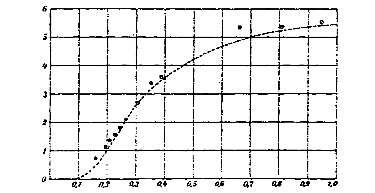
FIGURE \(24.\) Original figure from page 186 of ref.\(^{6}\), displaying no x-axis and y-axis labels.
FIGURE \(25.\) Table shown on page 190 of ref.\(^{6}\)
The values of temperature \(T\), which are seen in the first column, are recalculated and placed in the third column in the form of \(\frac{kT}{h\nu} = 0.00076 \ T\) for the specific value of \(\nu = 2.72 \times 10^{13} [Hz]\). The latter are the x-axis values in FIGURE 24. The interesting moment is how the frequency \(\nu\) value is determined, a value necessary to be plugged into the argument \(\frac{kT}{h\nu}\) in the curve-fitting formula.
This is what is donefirst, it is determined from the theoretical graph; that is, from the graph of the curve-fitting expression \(c_{curve-fitted} = 3R\frac{\left(\frac{h\nu}{kT}\right)^2 e^{\frac{h\nu}{kT}} }{ \left( e^{\frac{h\nu}{kT}} - 1\right)^2}\) as a function of \(\frac{kT}{h\nu}\), what the value of \(x = \frac{h \nu}{kT}\) is for a given, known from experiment, \(c_{experimental}\) value, as per the instructions of paper\(^{6}\), cited here.
Notice again, the approximating formula \(c_{curve-fitted} = 3R\frac{\left(\frac{h\nu}{kT}\right)^2 e^{\frac{h\nu}{kT}} }{ \left( e^{\frac{h\nu}{kT}} - 1\right)^2}\) which contains \(\frac{kT}{h \nu}\) as the independent variable, is most nonchalantly used to make a connection between a \(c_{experimental}\) value and the concrete expression, expression \(\frac{kT}{h \nu}\) (expression referring to a concrete value of \(\nu\)), completely unassociated with this \(c_{experimental}\) value.
This is presuming that because there is a functional connection between \(c_{curve-fitted} = 3R\frac{\left(\frac{h\nu}{kT}\right)^2 e^{\frac{h\nu}{kT}} }{ \left( e^{\frac{h\nu}{kT}} - 1\right)^2}\) which contains \(\frac{kT}{h \nu}\) and a \(\frac{kT}{h \nu}\) containing a concrete \(\nu\), then this proves that the same connection exists between \(c_{experimental}\) and \(\frac{kT}{h \nu}\), containing that same concrete \(\nu\). Such thing, however, cannot be presumed, because it is exactly what must be proved; namely, it must be proved that the concrete \(c_{experimental}\) is indeed connected with \(\frac{kT}{h \nu}\) containing that particular \(\nu\), not with \(\frac{kT}{h \nu}\), containing some other value of \(\nu\).
Thus, if you have obtained the value of \(\lambda = 1.1 \times 10^{-5}\) (\(\nu = \frac{c}{\lambda} = \frac{299792458}{1.1 \times 10^{-5}} = 2.72539 [Hz]\)) from the given \(c_{experimental} = 1.838\) for \(T = 331.3\), respectively, from \(x = \frac{kT}{h \nu} = 0.25\), then, of course, plugging that \(\lambda = 1.1 \times 10^{-5}\) back into \(\frac{kT}{h \nu}\) will recover the value \(c = 1.838\) for \(T = 331.3\), respectively, for \(x = 0.25\). This circular argument, however, does not prove that the experimental data have been recovered theoretically, and that the formula \(3R \frac{\left(\frac{h\nu}{kT}\right)^2 e^{\frac{h\nu}{kT}} }{ \left( e^{\frac{h\nu}{kT}} - 1\right)^2}\) predicts the experimental data.
The above fallacy very much resembles the deceptive proving, practiced in many a university, that the theory of relativity is not internally contradictory, because the Lorentz transformations purportedly are not internally contradictory. And, how does that proof work? Well, the conniving instructor applies the Lorentz transformations on a set of coordinates in one coordinate system, outright lying to the students that this is how the coordinates must look in another coordinate system. Then, to prove internal consistency, the irresponsible instructor applies the inverse Lorentz transformations on the deformed coordinates in the other system and recovers the initial coordinates, belonging to the first coordinate system. This is a classical case of deception in teaching and practicing of science. What the instructor must unquestionably do, if there is even a trace of integrity left in him, is to address first the flaws in the Lorentz transformations themselves. The instructor must tell the students that, in the first place, the Lorentz transformations themselves are mathematically crooked constructs because they presume that a constant is equal to a variable. Then the instructor must present to students what disastrous state of the matter the Lorentz transformations bring science to, by referring the students to the argument here. More on the matter can be read in my previous books, listed here.
If we use for the purpose of proving the predicting power of the curve-fitted expression, the straightforward \(c_{experimental}\) vs. \(T\) dependence taken from previously published tables, as the author of paper\(^{6}\) himself confides, we will again get nowhere, because even if we find the \(c_{experimental}\) for a given \(T\), this will carry no information about \(\lambda = \frac{c}{\nu}\) value and overlaying the \(c_{curve-fitted}\) graph over the experimental \(c_{experiment}\) points will only occur by patching the value of \(\nu\), until the curve of \(c_{curve-fitted} = 3R\frac{\left(\frac{h\nu}{kT}\right)^2 e^{\frac{h\nu}{kT}} }{ \left( e^{\frac{h\nu}{kT}} - 1\right)^2}\) finally falls onto the experimental \(c_{experimental}\) values.
Over and above all this insurmountable hurdle, even if we suppose that we have found a way to find the necessary \(\lambda = \frac{c}{\nu}\) from the \(c_{experimental}\) vs. \(T\) dependence, even then, the using of that experimentally found \(\lambda = \frac{c}{\nu}\) will do us no good in our strive to prove that our purportedly theoretically derived expression \(3R \frac{\left(\frac{h\nu}{kT}\right)^2 e^{\frac{h\nu}{kT}} }{ \left( e^{\frac{h\nu}{kT}} - 1\right)^2}\) predicts the outcome of the experiment. The value of the \(c_{experimental}\) will be recovered by the theoretical curve \(3R \frac{\left(\frac{h\nu}{kT}\right)^2 e^{\frac{h\nu}{kT}} }{ \left( e^{\frac{h\nu}{kT}} - 1\right)^2}\) no matter where on the graph the theoretical curve will be positioned. However, there is only one position of the theoretical curve, which makes it overlay the experimental curve. That special, unique position of the experimental curve is determined exclusively by the value of \(\lambda\) (respectively, \(\nu\)). However, in order for this to qualify as scientific derivation, the value of that \(\lambda\) (respectively, \(\nu\)) must not come from experiment. Predicting the outcome of an experiment by using the result of that same experiment, whose outcome we are supposed to predict, is nothing other than the logical fallacy known as petitio principii, a signature sign of bad science, sadly, a bad signature so much beloved by the destroyed science of today.
Question concerning the legitimacy of the critique
How come, you claim that the physics behind \(\overline{\varepsilon} = \frac{h \nu}{e^{\frac{h\nu}{kT}} - 1}\) is non-existent, but it happens to give a result, coinciding with experimental data?
The thing is, on the contrary, what is done in ref.\(^{6}\), on top of it, ill-begotten as early as ref.\(^{1}\), has nothing to do with physics. Paper\(^{6}\) comes up with a formal correction of Dulong and Petit formula \(c_v = 3R\) by curve-fitting a correction factor, because the experimental data for the specific heat of some elements is seen to exhibit a particular anomaly. Why this anomaly occurs, paper\(^{6}\) is unable to explain, although it launches itself into completely unsustained speculations about the physical side of a formula, which ref.\(^{6}\) could not even derive (neither could its originator Planck\(^{1}\), as seen here).
Therefore, if one is to seek the answer to the anomalous specific heat behavior of some elements in the quantum character of nature, that answer lies in the studies of C. I. Noninski, based on his view regarding the classical origin of \(\overline{\varepsilon} = \frac{h \nu}{e^{\frac{h\nu}{kT}} - 1}\), a view which differs radically from what is considered a view, albeit unjustified at all, expressed by Planck (cf. here). Plancks formula and C. I. Noninskis formula are similar in appearance but have an entirely different meaning. More precisely, Plancks formula lacks physical meaning, and is just a curve-fitting construct, as are the attempts, unsuccessful even as curve-fitting, such as the attempt of the author of ref.\(^{6}\) to apply Plancks formula in cases other that electromagnetic waves. The true meaning of \(\overline{\varepsilon} = \frac{h \nu}{e^{\frac{h\nu}{kT}} - 1}\) is put forth by C. I. Noninski, having at its basis the notion of exchanging energy (heat).
An aid to better understand the discussed curve
As an
aid to better understand the discussed curve, observe that it has the
shape of the function \(\frac{\left( \frac{1}{x} \right)^2
e^{\frac{1}{x}} }{ \left( e^{\frac{1}{x}} - 1\right)^2}\) when plotted
against \(x\), which is the reciprocal of \(\frac{1}{x}\). This plot
you may see for yourself in Wolfram Alfa on the net
\begin{equation*}
\scriptsize
\verb|plot ((1/x)^2 exp(1/x))/((exp{1/x} - 1)^2) |
\end{equation*}
\begin{equation*}
\scriptsize
\verb|for x = 1 to x = 10 |
\end{equation*}
\begin{equation*}
\scriptsize
\verb| plot ((1/x)^2 exp(1/x))/((exp{1/x} - 1)^2), |
\end{equation*}
\begin{equation*}
\scriptsize
verb|((1/(2x))^2 exp(1/(2x)))/((exp{1/(2x)} - 1)^2) |
\end{equation*}
\begin{equation*}
\scriptsize
verb|for x = 1 to x = 10 |
\end{equation*}
Even the triviality of curve-fitting is not utilized well
The
dimensionless factor \(3\frac{\left(\frac{h\nu}{kT}\right)^2
e^{\frac{h\nu}{kT}} }{ \left( e^{\frac{h\nu}{kT}} - 1\right)^2}\)
correcting \(R\) in the expression \(c =
3R\frac{\left(\frac{h\nu}{kT}\right)^2 e^{\frac{h\nu}{kT}} }{ \left(
e^{\frac{h\nu}{kT}} - 1\right)^2}\), allowing for a quasi-Dulong and
Petit law, aimed at reflecting anomalous specific heats of solids, has
only a seeming resemblance to the expression \(\frac{h \nu}{e^{\frac{h
\nu}{k \theta}}- 1}\) for \(U\), (\(\overline{\varepsilon}\)), because
this dimensionless correcting factor can simply be found through
curve-fitting, involving a fudge-factor notwithstanding. The
curve-fitting, utilizing the properties of the exponential function in
suitable combinations, a procedure of applied mathematics, not
associated in any way with \(\frac{h \nu}{e^{\frac{h \nu}{k \theta}}-
1}\), yields an expression \(5.94\frac{\left(
\frac{1}{x}\right)^2e^{\left( \frac{1}{x}\right)}}{\left(e^{\left(
\frac{1}{x}\right)} - 1\right)^2}\), which, plotted against \(x\),
would resemble the shape of the experimental \(c_{experimental}-T\)
data.
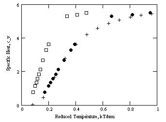
FIGURE \(26.\) The expression \(5.94\frac{\left( \frac{1}{x}\right)^2e^{\left( \frac{1}{x}\right)}}{\left(e^{\left( \frac{1}{x}\right)} - 1\right)^2}\), result of curve-fitting, plotted with + symbol, against \(x\), spanning from \(0\) to \(1\), the same span which the experimental data for the specific heats of diamond from the second column of the Table shown on page 190 of ref.\(^{6}\) (which is TABLE 16 shown here) when plotted against \( \frac{kT}{h\nu}\) for \(\nu = 2.72 \times 10^{13} [Hz]\), shown with solid circles. The empty squares indicate the same data taken from the second column of TABLE 16 here, plotted against \(\frac{kT}{h\nu}\) but this time for \(\nu = 5.44 \times 10^{13} [Hz]\).
The coincidence, practically, in FIGURE 26 (replica of the original FIGURE 24 of the data denoted by + (data obtained from the curve-fitted formula \(5.94\frac{\left( \frac{1}{x}\right)^2e^{\left( \frac{1}{x}\right)}}{\left(e^{\left( \frac{1}{x}\right)} - 1\right)^2}\)) with the data denoted by the solid circles (experimental data plotted against \(\frac{kT}{h\nu}\) for \(\nu = 2.72 \times 10^{13} [Hz]\)) is only due to the fact that the span of the independent variable \(x\) of \(5.94\frac{\left( \frac{1}{x}\right)^2e^{\left( \frac{1}{x}\right)}}{\left(e^{\left( \frac{1}{x}\right)} - 1\right)^2}\) was deliberately made to coincide with the span of the x-axis values corresponding to the particular \(\nu = 2.72 \times 10^{13} [Hz]\), against which the experimental solid-dot-data are plotted. However if the experimental data (shown in empty squares) are plotted against \( \frac{kT}{h\nu}\), calculated for \(\nu = 5.44 \times 10^{13} [Hz]\), it is clearly seen that these experimental data do not coincide at all with the points calculated from the formula \(5.94\frac{\left( \frac{1}{x}\right)^2e^{\left( \frac{1}{x}\right)}}{\left(e^{\left( \frac{1}{x}\right)} - 1\right)^2}\). Therefore, coincidence can only occur, if the span of the curve-fitted functions independent variable is known ahead of time, and the x-axis of the experimental points is adjusted through varying the frequency \(\nu\) to fit accordingly.
In other words, we are expecting the corrected Dulong and Petit to have the form \(c(T) = 3R.f(T)\), where \(f(T)\) is a correction coefficient to provide for the observed anomalously lower values of \(c\) at relatively lower \(T\). However, instead, a formula is obtained, which is a function of two variables \(c(T) = 3R.f(T, \nu)\). The frequency \(\nu\) is characteristic of each studied element, and the author of ref.\(^{6}\) proposes that \(\nu\) be determined by using a value of \(c\) already known from experiment, to become common for both the experimental and the curve-fitted data, so that \(\nu\) is eliminated from \(c(T) = 3R.f(T, \nu)\). So, in trying to prove that a formula agrees with experiment, the author of ref.\(^{6}\) uses what is known from experiment to prove the agreement with experiment. This is nothing other than petitio principii and constitutes no science at all.
Therefore, ref.\(^{6}\) does not have much to offer even as a curve fitting techniquepresenting graphically an expression obtained through curve-fitting, which displays the same shape as the shape formed by the experimental data, but finds a different position on the graph, depending on what frequency is plugged into the expression, and when choosing one concrete frequency of these arbitrary frequencies, having the available experimental values overlaid at the points of their abscissa position, calculated from that chosen frequency.
ADDENDUMDetails concerning specific heats of solids\(^{7}\)
In order to understand why the ratio \(\frac{\int Ee^{-\frac{N}{RT}E} \omega(E) dE}{\int e^{-\frac{N}{RT}E} \omega(E) dE }\) on the left side of the equality, shown as eq.(\ref{incorrectequality}) here (presented on page 138 of ref.\(^{7}\)), under the condition imposed by eq.(\ref{acondition}), is not equal to the right side of the purported equality, as said, presented here as eq.(\ref{incorrectequality}), cannot have anything to do with Plancks blackbody formula, consider the following simplified mathematical example:
Let us have a function \(f(x)\) such that \begin{equation}\label{condition} \int\limits_{\varepsilon}^{\varepsilon + a} f(x)dx = \int\limits_{2\varepsilon}^{2\varepsilon + a} f(x)dx ... = \int\limits_0^a f(x)dx = const, \end{equation} where \(\varepsilon\) is some small constant value of \(x\) and \(a\) is infinitesimally small. In other words, \(f(x)\) will have non-zero values only in the neighborhood of integer \(x\). For all other values of \(x\), function \(f(x)\) will be zero.
Now, we need the value of the integral \begin{equation}
\int\limits_0^n e^{-x} f(x) dx, \end{equation} as well as the value of
the integral \begin{equation} \int\limits_0^n xe^{-x} f(x) dx,
\end{equation} and the value of the quotient of the latter integral
over the former integral.
SolutionFirstly, as far as function \(f(x)\) goes, we make the
observation that there can be no other function but function \(f(x) =
const\), that can satisfy the condition expressed by
eq.(\ref{condition}). Therefore, \(f(x)e^{x}\) should in fact be
\(const . e^{x}\), and this we denote by the new function \(F(x)\).
So, \begin{equation} \int\limits_0^a e^{-x} f(x) dx = \int\limits_0^a
e^{-x} \ const\ dx = const \ \left( e^a - 1 \right). \end{equation}
Further, if the obtained \(\int\limits_0^a e^{-x} f(x) dx = c (e^{-a}
- 1)\), then, by the same token \(\int\limits_0^a xe^{-x} f(x) dx = c
ae^{-a}\). Thus, \(\frac{\int\limits_0^a xe^{-x} f(x)
dx}{\int\limits_0^a e^{-x} f(x) dx } = \frac{c \left( 1 - ae^{-a} -
e^{-a} \right) }{c\left(e^{-a} - 1\right)} = \frac{e^a - a - 1}{1 -
e^a}\) but it still seems indeterminate; i.e., something like
\(\frac{0}{0}\).
To solve this indeterminacy, we use the LHospital Rule (LHôpitals Rule) to find the limit at \(a \rightarrow 0\) \begin{equation} \lim_{a \rightarrow 0} \frac{e^a - a - 1}{1 - e^a} = \lim_{a \rightarrow 0} \frac{e^a - 1}{-e^a} = \frac{0}{-1} = 0. \end{equation} This solution, however, has nothing to do with Plancks law.
ADDENDUMImmediate proof that the theory in ref.\(^{7}\), regarding specific heats of solids, is wrong
In order to conclude that the author of ref.\(^{7}\) has not been able to derive the blackbody radiation formula, we need to understand exactly what he has done in his paper.
Thus, firstly, he attempts to develop some sort of a molecular-kinetic theory of heat. Erroneously thinking that he has found a truly realistic molecular-kinetic theory of heat by which some difficulties obstructing the implementation of that theory can be eliminated, he attempts applying it for a derivation in the theory of radiation, exemplified by Plancks formula.
On page 182 of ref.\(^{7}\), however, its author concludes that the molecular-kinetic theory developed by him only leads to the deficient Rayleighs formula \(\rho_{\nu} = \frac{R}{N} \frac{8\pi \nu^2}{c^3}T\) (eq.(6) in ref.\(^{7}\)); that is, it leads to the deficient known form \(\rho_{\nu} = \frac{8\pi \nu^2}{c^3}kT\) of Rayleighs formula. Just as a reminder, refer to footnote\(^{73}\) for an explanation why Rayleighs formula is deficient.
Therefore, the author of ref.\(^{7}\) eventually concludes the above, while, at the same time, correctly considering the fact that the formula \(\rho_{\nu} = \frac{8\pi \nu^2}{c^3} \overline{\varepsilon}\) must be retained. Even in this book, we talked a lot about the inevitability of that formula. The author of ref.\(^{7}\) assumes that it is the application of the molecular-kinetic theory, which causes a conflict with experience. Now, here, we must remark emphatically that it is his own attempt at molecular-kinetic theory, not the correct molecular-kinetic theory, that is not only causing conflict with experience, but is outright non-physical.
However, there is a much shorter way to see its invalidity, sparing the effort of analyzing every one of its premises. Thus, one can at once see that the theory proposed in ref.\(^{7}\) is incorrect, by observing that the ratio (the quotient), seen as part of eq.(4) on page 182 of ref.\(^{7}\) \begin{equation}\label{incorrectintegralquotient} \frac{\int{E e^{-\frac{N}{RT}E}}dE}{\int{e^{-\frac{N}{RT}E}}dE}, \end{equation} is not equal to \(\frac{RT}{N}\) but is equal to \(E + \frac{RT}{N}\). One may see this without delay by plugging \begin{equation*} \scriptsize \verb|(int (xe^(-(N/(RT))x))dx)/(int (e^(-(N/(RT))x))dx)| \end{equation*} into Wolfram Alpha on the net.
Therefore, when combining eq.(4) and eq.(5), known from Planck, the outcome is not \(\rho = \frac{N}{R} \frac{8 \pi \nu^2}{c^3}T\) (replacing \(L\) with \(c\) as the symbol of the speed of light), claiming recovery of Rayleighs formula, but is \begin{equation} \rho = E\frac{8 \pi \nu^2}{c^3} + \frac{N}{R} \frac{8 \pi \nu^2}{c^3}T, \end{equation} which differs from Rayleighs formula by the term \(E\frac{8 \pi \nu^2}{c^3}\).
In other words, the theory which the author of ref.\(^{7}\) proposes cannot recover even the rudimentary Rayleighs formula.
As an aside, recall that Rayleighs formula \(\rho = \frac{8 \pi \nu^2}{c^3}kT\), where \(k = \frac{N}{R}\), incorrectly represents the spectral energy density distribution as the curve depicting this distribution approaches the lower wavelengths; that is, the higher energies in the ultraviolet region and beyond. This leads to the ultraviolet catastrophe because of the non-physical acceptance that the mean energy per resonator referring to the total system can be assigned equally to all resonators, albeit each one with its different frequency.
From that moment on; that is, from page 183 of ref.\(^{6}\) on, we can proceed with the analysis in the main text, which, unfortunately, will also reveal that the goal stated at the beginning of ref.\(^{7}\)modification of the molecular-kinetic theory of heat, is also unsuccessful. This modification not only does not eliminate the inferred some difficulties obstructing the implementation of that theory, but makes no sense at all.
\( \LARGE \mathbb{COMES \ TO \ THE \ RESCUE}\)
CLASSICAL DERIVATION OF THE SPECTRAL ENERGY DENSITY OF BLACKBODY RADIATION BY C. I. NONINSKI
Now, we
are ready to move on and dive into the most interesting part of our
exposé.
C. I.
Noninskis derivation\(^{11}\) (cf. the
facsimile here) is based on the
following prerequisites:
\(\bullet\)
The heat motion of the particles of a thermodynamic system is modeled
by the periodic motion of a simple harmonic oscillator. Recall,
Plancks model\(^{1}\) observes the induced
periodic motion of a collection of resonators, which, principally,
does not make a difference, compared to C. I. Noninskis simple
harmonic oscillator model.
\(\bullet\)
A simple harmonic oscillator (resonator), isolated from its
environment has the mean energy \(\overline{\varepsilon} = 2 \pi^2 A^2
m \nu^2\). See the notation and the derivation
of this expression.
\(\bullet\)
When the isolation around an oscillator is removed, because of the
exchange with the other oscillators, there are three sorts of energy
quantities:
1. Average (mean) energy of the oscillator \(\overline{\varepsilon}\)
2. Freely exchanging (and transforming, to be exact) fluctuation
energy \(\Delta \varepsilon\), which is distributed ideally randomly
amongst the oscillators.
3. residual energy of the oscillator \(\varepsilon_{(-)}\)
Probably one of the most important observations made in C. I. Noninskis paper\(^{11}\) is that there is a difference between the way the phenomenological classical thermodynamics views energy of the particle, as well as the notions work and heat, on the one hand, and the treatment of these quantities in statistical mechanics. Classical thermodynamics, unlike statistical thermodynamics, never confuses energy of the particle with the exchanging part of that particles energyheat and work. Unlike statistical mechanics, when a process is observed in classical thermodynamics, it is only connected with the exchanging part of the energy, which is nothing other than heat.
Once
this is understood, then it further has to be absorbed that
the mean fluctuation \(\overline{|\Delta \varepsilon|}\) from the mean value \(\overline{\varepsilon}\) is very specifically related to that mean value \(\overline{\varepsilon}\) in this particular sort of a problem. This problem involves the Poisson energy distribution, which is the distribution in a system consisting of discrete elements. We will not go into the details of this kind of distribution but will employ one extremely important property it possesses, when it comes to the problem at hand; namely, that in systems in which the energy of their particles is characterized by Poisson distribution, it is very unlikely for a particle to lose all of its energy content and transfer it to another particle, as a result of random fluctuation of its energy. On the contrary, and that is the really astonishing property of the Poisson distribution, the average fluctuations of the energy around the mean energy of the particle, constitute only an amount equal to none other than the variance; that is, the square of the standard deviation, characterizing the fluctuations \(\Delta \varepsilon\) around the mean value \(\overline{\varepsilon}\) \begin{equation}\label{meansquareoffluctuation} \overline{(\Delta{\varepsilon})^2} = \overline{\varepsilon}, \end{equation} where the so-called variance \(\overline{(\Delta{\varepsilon)}^2}\) around the mean value \(\overline{\varepsilon}\) (\(\overline{\varepsilon}\) is a value we already derived here), is the mean square of the fluctuation \(\Delta{\varepsilon}\). Eq.(\ref{meansquareoffluctuation}) follows from the so-called index of dispersion (cf. ref.\(^{29}\)), whereby the quotient of the variance \(\overline{(\Delta{\varepsilon)}^2}\) and the mean value \(\overline{\varepsilon}\) of the particle energy, is unity for phenomena, such as the Brownian motion or radioactive decay, involving a collection of separate entities.
In other words, the standard deviation, the spread, the mean value of the fluctuations \(\Delta \varepsilon\) around the mean value \(\overline{\varepsilon}\), are equal to the square root of that mean value \(\overline{\varepsilon}\); that is, to \(\sqrt{\overline{\varepsilon}}\).
The property of the Poisson distribution expressed by eq.(\ref{meansquareoffluctuation}), provides the amazing opportunity to connect the calculable average energy content \(\overline{\varepsilon}\) of the oscillator (cf. here) with the variance, \(\overline{(\Delta{\varepsilon})^2}\), expressed by the mean values of the square of the unknown fluctuations of energy around this average energy content. This role of variance is hardly ever utilized, the instructors practically always using variance as the stepping stone to talking about standard deviation. In the discussed case, we also make the transition variance\(\rightarrow\)standard deviation, but we never forget that, now, this standard deviation is, in fact, the sought for average exchanging heat, the knowledge of which makes all the difference in our quest for finding the classical expression describing the spectral energy radiation density of a blackbody.
We may express eq.(\ref{meansquareoffluctuation}) in a dimensionless form by dividing the \(\varepsilon\) on both sides of eq.(\ref{meansquareoffluctuation}) by some constant energy value of quantity \(\varepsilon_0\) \begin{equation*} \overline{\left( \Delta \frac{\varepsilon}{\varepsilon_0} \right)^2} = \overline{\left( \frac{\varepsilon}{\varepsilon_0} \right)} \end{equation*} \begin{equation*} \overline{\Delta \frac{\varepsilon^2}{\varepsilon_0^2} } = \overline{\left( \frac{\varepsilon}{\varepsilon_0} \right)} \end{equation*} \begin{equation*} \overline{\Delta \varepsilon^2} = \overline{\left( \frac{\varepsilon_0^2\varepsilon}{\varepsilon_0} \right)} \end{equation*} or \begin{equation}\label{variancefrommeanenergy} \overline{\Delta {\varepsilon}^2} = \varepsilon_0 \overline{\varepsilon}. \end{equation} The obtainment of eq.(\ref{variancefrommeanenergy}) is the central moment in the classical derivation of the spectral energy distribution of the blackbody emission. That equality enables us to assess the average quantity of energy (heat), which is being exchanged between the particles of the system, comprising exactly the quantity which is of interest for our discussion, from a quantity mean energy of the oscillator, \(\overline{\varepsilon}\), which we know how to calculate (cf. here).
From that moment on, having at hand eq.(\ref{variancefrommeanenergy}), which ensures that we know the average value of the exchanging energy (heat), the rest of the derivation follows a very straightforward, logical path, which utilizes the direct, tangible connection, through Boltzmanns distribution law, of the molecules with their exchanging energy, rather than seeking the indirect connection, through entropy, of this relation.
Now, it is instructive to see where we are heading. Our goal is to derive the correct expression; that is, the expression regarding exchanging energy, which will replace the incorrect presence of the mean energy \(\overline{\varepsilon}\) of the oscillator in the formula \(\frac{8 \pi \nu^2}{c^3}\overline{\varepsilon}\) (in Plancks paper having the form of \(\frac{8 \pi \nu^2}{c^3} U\)) for the spectral energy density of the blackbody radiation. This substitution of \(\overline{\varepsilon}\) with an expression for the average exchanging heat, is ensured by eq.(\ref{variancefrommeanenergy}), after some additional minimal steps.
So, from now on, we are aiming our focus at the average fluctuation \(\overline{|\Delta \varepsilon|}\), which can, obviously, be obtained from the pivotal equation (equation for the variance of the fluctuations of energy) \(\overline{\Delta {\varepsilon}^2} = \varepsilon_0\overline{\varepsilon}\), eq.(\ref{variancefrommeanenergy}), which, considering the expression for \(\overline{\varepsilon}\) derived here, becomes \begin{equation}\label{varianceappliedtofluctuation} \overline{\Delta {\varepsilon}^2} = \varepsilon_0\overline{\varepsilon} = \varepsilon_0 2 \pi^2 A^2 m \nu^2, \end{equation} from where, the mean square fluctuation (the standard deviation) of the oscillator energy is \begin{equation}\label{meanabsolutevalueoffluctuation} \sqrt{\overline{\Delta {\varepsilon}^2}} = \sqrt{\varepsilon_0\overline{\varepsilon}} = \pi A \sqrt{2 m \varepsilon_0} \ \nu. \end{equation} This equation, eq.(\ref{meanabsolutevalueoffluctuation}), is the mean exchanging energy (heat).
Now, for simplicity, in order not to get into the trivialities of statistics, not at issue in this context, we will adopt that the above-shown eq.(\ref{meanabsolutevalueoffluctuation}) approximately expresses the mean absolute value of the fluctuation \(\overline{|\Delta \varepsilon|}\) (cf. footnote\(^{74}\))the central quantity of interest in the current derivationas \begin{equation}\label{newquantum} \overline{|\Delta \varepsilon|} = \mathscr{h} \nu, \end{equation} where \( \mathscr{h} = \pi A \sqrt{2 m \varepsilon_0} \) is a constant.
Now, using the expression \(\mathscr{h} \nu\) from eq.(\ref{newquantum}), which gives the average value of one-oscillator-exchanging-energy-portion, transported amongst the oscillators, it is easy to calculate the mean value of the exchanging energy (heat) \(\overline{\Rule{0em}{0em}{0em}\smash{\mathscr{q}}} \, \, \), corresponding to one oscillator of frequency \(\nu\).
A word of warning\(\mathscr{h} \nu\) is the average (classical) quantum of exchanging heat one oscillator loses, going out to the rest of the oscillators, if that oscillator happened to give off energy, as are the already defunct chunks (quanta) \(h\nu\) of the quantity \(U\), which Planck erroneously designates as the average energy of one resonator. Because not all oscillators participate in that exchange, the overall exchanging heat \(\overline{\Rule{0em}{0em}{0em}\smash{\mathscr{q}}} \, \, \) per oscillator, calculated by including the oscillators that did not give off energy, the object of our forthcoming derivation, will be less than \(\mathscr{h} \nu\).
Thus, as just said, in the following paragraphs, our goal will be to derive the expression for the quantity \(\overline{\Rule{0em}{0em}{0em}\smash{\mathscr{q}}} \, \, \), comprising the mean exchanging energy (heat) per oscillator, observing what the connection is between \(\overline{\Rule{0em}{0em}{0em}\smash{\mathscr{q}}} \, \, \) and the tiny elementary chunks of exchanging energy \(\mathscr{h} \nu\).
Before that, we may note that one should appreciate the natural way,
in which the quantum condition \(\overline{|\Delta \varepsilon|} =
\mathscr{h} \nu\) is arrived at classically, without the need to
resort to postulates coming out of thin air. Besides, the arbitrary
division by Planck of Plancks \(U\) into uniform chunks \(\varepsilon
= h \nu\) of energy, \(U\) being a quantity not only confused by
Planck, but a quantity that cannot even be reached, because of the
earlier collapse of Plancks theory itself anyway, is represented in
the classical derivation by averaging irregular portions of \(\Delta
\varepsilon\) exchanging energy (heat) among oscillatorscf. herewhose
average is \(\mathscr{h} \nu\). Consider also this quotation from C. I
Noninski\(^{11}\):
Planck
observes the total energy \(U_N\) of all \(N\) oscillators of
frequency \(\nu\) as divided into equal parts(energy elements,
quanta), each one equal to \(\varepsilon\). However, this is only
one formal acceptance with the aim to solve the problem of finding
the most probable distribution of this energy among the oscillators.
In reality, as is seen from the derivation of (11), Planck would
have obtained exactly the same result if he had accepted that the
energy \(U_N = NU\) is not divided into equal parts but is divided
into arbitrarily sized parts, as a re the actual fluctuation of the
energy of the oscillator, and then would have taken the average
value of these variously sized energy portion (fluctuations). In
other words, Plancks elementary quantum of energy is none other
than the mean value of the fluctuations of the energy of an
oscillator having a given frequency vibrations.
With this remark out of the way, we are now ready to proceed with the promised derivation.
Thus, let the total number of resonators be \(1\) mole (Avogadros number) of resonators, which we will denote by \(N\). Then, with Boltzmann, the number of molecules (particles, oscillators) that have acquired the additional average energy due to transfer of average heat in the amount of \(\mathscr{h} \ \nu\), is \(N e^{-\frac{\mathscr{h} \ \nu}{kT}}\).
Notice once again, that \(\mathscr{h} \ \nu\) is, as said, the average exchanging energy (heat) per oscillator, which the oscillator did gave off to the rest of the oscillators (some oscillators did not give off this quantum of energy). The quantity \(\mathscr{h} \ \nu\) participates in the calculation of \(\overline{\Rule{0em}{0em}{0em}\smash{\mathscr{q}}} \, \), which is the focus of C. I. Noninskis derivation. It is this \(\mathscr{h} \ \nu\) chunk that makes the character of that derivation acquire the qualifier quantum completely classically and naturally. Therefore, the probability that \(1\) oscillator will possess that excess energy \(\mathscr{h} \ \nu\), through acquiring that portion \(\mathscr{h} \ \nu\) of exchanging heat from another oscillator, is \(e^{-\frac{\mathscr{h} \ \nu}{kT}}\). Then, \(Ne^{-\frac{\mathscr{h} \ \nu}{kT}}\) will be the probability that \(N\) oscillators will possess that excess energy (energy above the mean energy \(\overline{\varepsilon}\)) \(\mathscr{h} \ \nu\). Hence, the above \(Ne^{-\frac{\mathscr{h} \ \nu}{kT}}\) number of oscillators will possess excess energy amounting to \begin{equation} \mathscr{h} \ \nu N e^{-\frac{\mathscr{h} \ \nu}{kT}}. \end{equation} Thus, the fraction \(Ne^{-\frac{\mathscr{h} \ \nu}{kT}}\) of the oscillators that have acquired that excess exchanging heat, out of all the total of \(N\) oscillators, subtracted from that total number \(N\) of oscillators, gives the remaining number of oscillators \(N - Ne^{-\frac{\mathscr{h} \ \nu}{kT}}\) which have not acquired that excess exchanging heat \(\mathscr{h} \ \nu\). On the contrary, these \(N - Ne^{-\frac{\mathscr{h} \ \nu}{kT}}\) oscillators, together, constitute the donor of the observed excess exchanging energy (some of these member-oscillators of the donor have given off quantum \(\mathscr{h} \ \nu\) of energy (heat), some have not).
Now,
because the \(Ne^{-\frac{\mathscr{h} \ \nu}{kT}}\) of the oscillators
which have acquired the excess exchanging heat could not have any
other source for that acquired excess exchanging heat, than from the
remainder \(N - N e^{-\frac{\mathscr{h} \ \nu}{kT}}\) of the
oscillators, then the exchanged energy (heat) \(\overline{q} \, \, \)
per oscillator must be the quotient, having as the numerator the total
excess exchanging heat \(\mathscr{h} \ \nu N e^{-\frac{\mathscr{h} \
\nu}{kT}}\) which the \(N e^{-\frac{\mathscr{h} \ \nu}{kT}}\)
oscillators possess, and as the denominator, the remainder of the
oscillators \(N - N . e^{-\frac{\mathscr{h} \ \nu}{kT}}\) that have
given off their energy in the form of heat and now are deficient (some
of them) in this energy. Therefore, the average exchanging heat
\(\overline{q}\) per every single oscillator will be \begin{equation*}
\frac{\mathscr{h} \ \nu N e^{-\frac{\mathscr{h} \ \nu}{kT}}}{N - N
e^{-\frac{\mathscr{h} \ \nu}{kT}}}, \end{equation*} which, after
cancellation of \(N\) and division of both numerator and denominator
by \(e^{-\frac{\mathscr{h} \ \nu}{kT}}\), becomes \begin{equation*}
\frac{\mathscr{h} \ \nu e^{-\frac{\mathscr{h} \ \nu}{kT}}}{1 -
e^{-\frac{\mathscr{h} \ \nu}{kT}}} \end{equation*} \begin{equation*}
\frac{\mathscr{h} \ \nu \frac{e^{-\frac{\mathscr{h} \
\nu}{kT}}}{e^{-\frac{\mathscr{h} \
\nu}{kT}}}}{\frac{1}{e^{-\frac{\mathscr{h} \ \nu}{kT}}} -
\frac{e^{-\frac{\mathscr{h} \ \nu}{kT}}}{e^{-\frac{\mathscr{h} \
\nu}{kT}}}} \end{equation*}
\begin{equation}\label{generalexponentialfactor} \frac{\mathscr{h} \
\nu }{e^{+\frac{\mathscr{h} \ \nu}{kT}} - 1}. \end{equation}
Eq.(\ref{generalexponentialfactor}) will undergo further
specification, especially in C. I. Noninskis derivation, where the
quantum of energy \(\mathscr{h} \ \nu\), classically derived, which
Plancks derivation cannot justify, in spite of the widely acclaimed,
in fact, non sequitur postulation that \(\varepsilon = h
\nu\), will find its clear classical meaning.
Cut-off point
When it comes to understanding of certain matters in general, but especially in science, one not only limits oneself to certain notions, but one comes to realize what exactly the notions advancing that understanding are, and what notions are secondary and can even be ignored for the time being. Once the essence of the problem is understood under those truncated conditions, one is quite welcome to develop ones understanding by dwelling further into the intricacies of the problem. Such development is worthwhile only if the groundwork, the canvas, is properly established.
Thus, the discussion of the concrete form of the distribution to be contemplated may be postponed, realizing that, at least, it must be of discrete type; namely, a variant of the so-called Binomial distribution. The usual discrete distribution contemplated, is the Poisson distribution, known as being right-skewed, meaning that its graph is asymmetric, with the extended right tail. However, as the number of samples increases, it becomes more and more symmetric, resembling more and more a normal distribution.
This may become clear with an example. We denote the probability that an event will occur \(x\) times by symbolically writing \(P(X = x)\). Then, if the distribution is Poisson, we will have \begin{equation} P(X = x) = \frac{\mu^x \ e^{-\mu}}{x!}, \end{equation} where \(\mu\) is the entire population mean with standard deviation denoted by \(\sigma\) (as opposed to the sample mean \(\overline{x}\), characterized by standard deviation denoted by \(s\); that is, the mean of only an extract from the entire population).
When we speak of distribution, first of all we think of a variable. Then, we imply a function of that variable, a function which establishes the number of occurrences of the variable.
Plancks blackbody radiation formula is a distribution. It is a function, which shows, so to say, how many occurrences; that is, how high the value of the function will be for every value of the variable \(\nu\).
It is extremely important to note here that the described classical way of deriving the blackbody radiation formula, now reveals very clearly the dependence of the energy in question, both on frequency \(\nu\), and on amplitude \(A\) of the wave.
The above classical expression \(\frac{\mathscr{h} \ \nu }{e^{+\frac{\mathscr{h} \ \nu}{kT}} - 1}\), eq.(\ref{generalexponentialfactor}), derived by C. I. Noninski, has the same form as Plancks eq.(11) of ref.\(^{1}\); namely, \(\frac{h \ \nu }{e^{+\frac{h \ \nu}{k \theta}} - 1}\). However, the former, \(\frac{\mathscr{h} \ \nu }{e^{+\frac{\mathscr{h} \ \nu}{kT}} - 1}\), has a real physical content, not just playing the role of a curve-fitting expression, as does the latter. The classical expression for the spectral energy density of blackbody radiation \(\rho_{\nu} = \frac{8 \pi \nu^2} {c^3}\overline{\Rule{0em}{0em}{0em}\smash{\mathscr{q}}} \ \) thus becomes \begin{equation}\label{ClassicalPlanckEquation} \rho_{\nu} = \frac{8 \pi \nu^2} {c^3} \frac{\mathscr{h} \nu} {e^{\frac{\mathscr{h}\nu}{k T}}-1}, \end{equation} where the value of the constant \(\mathscr{h}\ \) can be determined in the same way as it was determined by Planck in part \(3\) (\(\S11\) and \(\S12\) of ref.\(^{1}\), based on the experimental values found by Lummer and Pringsheim\(^{24}\) and others.
Further, eq.(\ref{ClassicalPlanckEquation}), \(\rho_{\nu} = \frac{8 \pi \nu^2} {c^3} \frac{\mathscr{h} \nu} {e^{\frac{\mathscr{h}\nu}{k T}}-1}\), derived here, coincides in appearance with Plancks eq.(12), \(u = \frac{8 \pi \nu^2} {c^3} \frac{h \nu} {e^{\frac{h\nu}{k \vartheta}}-1}\) in ref.\(^{1}\), which Planck could not even derive. Unlike Plancks equation, eq.(\ref{ClassicalPlanckEquation}) is derived quite elegantly, entirely classically.
Furthermore, equations \(\frac{\mathscr{h} \ \nu }{e^{+\frac{\mathscr{h} \ \nu}{kT}} - 1}\), eq.(\ref{generalexponentialfactor}), respectively, \(\rho_{\nu} = \frac{8 \pi \nu^2} {c^3} \frac{\mathscr{h} \nu} {e^{\frac{\mathscr{h}\nu}{k T}}-1}\), eq.(\ref{ClassicalPlanckEquation}), are based on the real meaning of the mysteriously postulated quantum of energy \(\varepsilon = h \nu\) (ref.\(^{1}\)), which now acquires its clear physical meaning, namely, the mean value of the exchanging energy fluctuations \(\varepsilon = \mathscr{h}\nu\) (eq.(\ref{newquantum}), respectively, eq.(\ref{MeanFluctuation})) (average energy portion, average heat, which the oscillators exchange among themselves), which classical thermodynamics refers to as heat.
As seen, Plancks formula for the elementary quantum \(\varepsilon = h \nu\) after the above classical derivation, is no longer an empirical formula, which Planck has postulated to describe radiation, as hitherto thought. Neither is it describing some new property of particles, unknown to classical physics. Plancks formula, which Planck actually failed to derive, is fully derivable classically and has a clear physical meaning (cf. eq.(\ref{newquantum}), respectively, eq.(\ref{MeanFluctuation})). Thus, it is noted in ref.\(^{11}\), that quantum mechanics is in fact classical mechanics when, correctly, the mean exchange energy (mean heat) of the particles is observed, instead of confusing it with the actual energy the particles themselves possess. Further, since energy is a state function of the system, one can speak of energy at a given moment only in such a case. However, the exchanging energy (heat, work) is always connected with the change of state; that is, with a process. The exchanged portions of energy cannot be transferred instantly, but the swap takes place within a finite time interval. Do you now see how naturally the uncertainty relation concerning energy and time comes about entirely naturally? It is exactly this impossibility to have exchanging energy (heat) transferred at a given moment of time, and therefore to have momentum of the particle at a given position of space, that is the most natural characteristic of the classical particlesclassical uncertainty principleunlike the impression created, that said principle is some unusual, inexplicable, property (uncertainty principle) of particles in some imaginary quantum mechanicsmore on this will be discussed latercf. here and here. Thus, the so-called quantum physics and quantum chemistry, in fact, study the interaction between particles, the fluctuations of mechanical motion (which is the fluctuation of their energy, their exchanging energy), not their mechanical motion itself (not the factual energy of the particles themselves). This correct understanding of quantum mechanics takes away its mystery, avoids the need for various interpretations and brings it back into the realm of reason and physical consistency of classical mechanics, as pointed out in the excerpt from C. I. Noninskis paper presented on .
On
a more general note, the main problem of contemporary physics, which
has backed it into a corner, is the incorrect view of motion,
respectively of interaction, describing motion through rest. This
wrong description of motion is inherent as early as Newtons second
law, used in its incomplete form even today. The problem is seen at
once when observing the DAlembert principle. The inadequate
description of motion through rest leads to the incorrect form of the
currently used Lagrangians and, respectively, Hamiltonians. That
causes part of the problems in the so-called quantum mechanics, in
addition to the above-discussed problems. All these considerations
will be the subject of future communications.
A short quotation from C. I. Noninski's paper, a facsimile of which is seen here
It will certainly be worth presenting, translated, a short quotation of a text from C. I. Noninskis paper\(^{11}\), whose facsimile is seen here. Of course, a full-translation into English of C. I. Noninskis paper\(^{11}\) is long overdue, and this author is urging those responsible for the archival scientific literature to fill this gap and publish in English this seminal paper, providing the initial impetus for the entire overturning of most of contemporary physics and chemistry.
Says C. I. Noninski in paper\(^{11}\) (its
facsimile is seen here):
As is seen, all facts point to M. Planck being able to manage explaining the spectral distribution of the black radiation thanks to the circumstance that, unlike all other students of this phenomenon, he, in fact, does not observe the energy of the oscillator but observes the fluctuations of this energy (the exchanging energy, the heat). However, on the other hand, just like the other students of the heat emission of an absolutely black body, he does not lay a clear boundary between these two notions and observes the mean exchanging (emitted) energy of the oscillator as the mean energetic state of that oscillator.
This weakness of Plancks study was later interpreted as its strongest side: the extremely great successthe derivation of the law of energy distribution in the spectrum of the absolutely black bodywas explained by the supposition that Planck had discovered unusual properties of the energy of the linear harmonic oscillator and of all particles, not by the simple fact that Planck was the first to observe the energy actually emitted by the oscillatorthe fluctuation energy (the heat). An entire theory was created about the purported special properties of the energy of the particlesthe old quantum theory, which evolved into quantum mechanics (and in the past decades quantum physics and quantum chemistry is being spoken of).
All attempts, however, to clarify the physical meaning of the quantum properties of the energy of the particles were doomed to fail in advance because, in actuality, it does not possess such properties; foreign properties were assigned to it; namely, the properties of exchanging energy, which is quantized to begin with: it consists of parts varying in magnitudethe fluctuations, whose mean value is a single-valued function of the frequency and at a given frequency is a constant quantityan elementary quantum of energy.
With the creation of quantum mechanics, in fact, the answer to the question was given as to what would classical mechanics look like if under the energy of the particles we would understand their heat (the exchanging energy) and not their factual energy.
It is known from thermodynamics that, while energy is the function of the state of the system and one can speak of energy of the system at any moment, the exchanging energy (the heat, the work) is always connected with change of the state of the system (with a process), because of which it always corresponds to a smaller or larger time interval, rather than to a given moment of time. Therefore, with considering of the exchanging energy (the heat) as energy of the particles, the possibility to speak of energy of the particles at a given moment, is at once excluded; one can only speak about energy corresponding to a given interval of time (during which the exchange of energy takes place). Exactly this impossibility to speak of energy of the particle at a given moment, and therefrom, about impulse of the particle at a given point of space, is one of the most characteristic features of quantum mechanics, which is expressed by the known Heisenberg uncertainty relations (inexactness): \begin{equation*} \Delta E \Delta t \approx h \end{equation*} and \begin{equation*} \Delta p_x \Delta x \approx h, \end{equation*} where \(E\) is the energy, \(t\) is time, \(\Delta p_x\) is impulse along the x-axis, \(x\) is a coordinate and \(h\) is Plancks constant.
From all said so far, it is seen that the quantum properties of the
particles are strange and incomprehensible only if they are being
connected to the energy of the particles; they become entirely
comprehensible, if they are observed as properties, connected with
the fluctuations of the energy of the particles (with their
exchanging energy). It
is also seen that the quantum area of physics and chemistry has, as
the object of study, the interaction between the particles (the
exchanging energy in its essence is energy of the interaction), not
the mechanical motion of the particles. One can speak of quantum
mechanics insofar as notions of classical mechanics are being used;
one must not forget, however, that the impulses and coordinates in
quantum mechanics provide, in the general case, the fluctuations of
the mechanical motion of the particles, not just their mechanical
motion.
C. I. Noninskis proof that Wien considers the oscillator as losing all its energy
We saw that the arrival at the correct form \(\rho_{\nu} = \frac{8 \pi \nu^2} {c^3} \frac{\mathscr{h} \nu} {e^{\frac{\mathscr{h}\nu}{k T}}-1}\), eq.(\ref{ClassicalPlanckEquation}), of the blackbody radiation formula, be it through the mathematical methods of curve-fitting, to resemble the experimentally established curve, or by whatever happenstance, through faulty adjustment of algebraic expressions (Planck), in fact, reflects, from a physical point of view, exchanging energy (heat). C. I. Noninski was the first to derive that formula from this correct physical prerequisite. He was also able to explain why Wiens distribution law does not quite coincide with the experimental curve. While Wien too, unbeknownst to him, derives a formula whose correct physical content is exchanging energy, he misinterprets the extent of that exchanging heat. C. I. Noninski demonstrates that Wiens formula is derived under the premise that when a resonator gives off its energy in the form of heat, Wien incorrectly considers that the oscillator in question releases its entire energy, remaining with zero net energy after that process.
Thus, if in the expression for the exchanging energy obtained by C. I. Noninski\(^{11}\), it is considered that all of the energy of the oscillator is exchanged, then such consideration will lead to exactly the obtainment of Wiens law. Correctly considered, as seen, it is only part of the energy of the oscillator that is transferred.
In other words, Wien does not connote the true exchanging energy, but what he implicitly, unknowingly considers as exchanging energy, is the entire energy of the oscillator. Indeed, if instead of the correct formula comprising the equation derived by C. I. Noninski, one applies the Boltzmann formula on a model, whereby one assumes that the energy of the resonators which have given off energy has become equal to zero, while the oscillators which have accepted energy only have the exchanging energy, equal to \(\varepsilon_{_1} = c_{_2} \nu\), then (using C. I. Noninskis notation), according to Boltzmanns law, the number of oscillators that have accepted energy (heat) \(c_{_2} \nu\) is \(Ne^{- \frac{c_{_2} \nu}{kT}}\). Therefore, the excess energy, accepted by the those oscillators that have it, is \(c_{_2} \nu Ne^{- \frac{c_{_2} \nu}{kT}}\). What Wien, in effect, does is divide that excess energy by the total number \(N\) of the oscillators \begin{equation*} \overline{\Rule{0em}{0em}{0em}\smash{\mathscr{q}}} \, \, = \frac{c_{_2} \nu N e^{- \frac{c_{_2} \nu}{kT}} }{N} = c_{_2} \nu e^{- \frac{c_{_2} \nu}{kT}}. \end{equation*} The above expression exactly coincides with the formula which Wien derives for the energy of the oscillator (cf. the equation on p.220 of Wiens original\(^{10}\), the facsimile here; cf. also here).
However, if we really accept that the denominator should be the total number of oscillators, that would mean that the number of the oscillators that are source for the excess energy comprising the numerator would be \(N e^{\frac{0}{kT}} = N.1\), the latter answering the question how many oscillators have remained that have lost all their energy; that is, how many oscillators have energy 0? in other words, Wiens law is arrived at as a result of the premise that all resonators have transferred all their energy. Therefore, the excess energy would comprise all the available energy of the oscillators, driving them to sheer energy poverty, an obviously non-physical assumption.
A bit of memory
Sometimes I wonder, what a thing life is. Nothing matches timewise. When you needed the arguments the most, you didnt have them, and when you have them, its too late. I happen to know someone personally, because he was a friend of my father and used to come and visit us. But, I was a child then and in my eyes he was a great hero. In truth, he was a very humble man and the fact that he knew someone, was not something that he would wave like a bannersomething that many others would, then, have stuck on their chest like a medal of distinction. My father had mentioned him, so thats how I know he was an assistant to some famous person. The question I ask myself today is, why was I the one, destined to show up and find what inadequacy that famous person in question had become famous for. Let alone that all the other works of that famous person, even those unrelated to relativity, turned out to be flagrant nonsense. Where were the likes of that friend of my father, to grasp what they were getting themselves into? I dont know. Is it opportunism, is it reverence for authority, that freezes thought? Is it purely riding on the momentum of someone completely wrongly recognized by the academia as genius, or is the reason somewhere else, so the likes of that otherwise very humble friend of my father didnt realize what an undignified game they were involved in playing? Things in the normal course of science, which are not at play in this case, are rooted in the nature of discovery. Can one blame Aristotle for not seeing the errors in his works, discovered later by Galileo? Unlike the natural course of science, which led Galileo to correct the errors of a predecessor, however, in the case of the one who pushed the absurd theory of relativity, whether he wrongfully presented it as his or not, we are talking about something unheard of and unprecedented, which is not even an error, but blatant lunacy. There is no example in the entire history of science of such absurdity, taking over science so brazenly, and on such a broad scale.
Why didnt C. I. Noninski continue his studies?
Everything on this matter, as in any matter having to do with creativity, is speculative, but one thing is for sure, anyone dealing with scientific critique of the particular absurdities, subject of attention in this book, pronounced, on top of it, as fundamentals, absurdities such as relativity and quantum mechanics, puts his life and the life of his family in jeopardy in any society under any regime. Relativity and quantum mechanics have attained such societal prominence on a global scale, that any thought of doubt is met with profound resentment by the entire system. These topics have soaked and penetrated society so deeply, that they now have become ubiquitous beyond religion and faith, the latter only limiting itself to enclaves and denominations. The critique of relativity and quantum mechanics, as rightfully proving the dramatic catastrophe of these undertakings, has a completely different place and character than any other critique in science. Relativity and quantum mechanics are not science. They are a cult. Partially, that cultification is due to major financial interests that have sedimented around these areas, grasping the imagination as unwieldy and incomprehensible but hauntingly esoteric, yet appearing justified as being figments of academia. On the other hand, it may not be at all unplausible, that the mass fascination with these absurdities, is due to their appearance as something different, interesting in its unlikeliness, which nevertheless has gained approval. No matter what the reason for their societal promotion might be, there are unequivocal facts that make these intellectual invaders all about really bad accidents that have dawned upon science. So far, we have devoted quite a few pages to the physical problems of these unseemly intruders, noting that one of them, relativity, must at once leave science altogether. The other, quantum mechanics, must return to its roots, classical mechanics, a major road for that return pointed to by C. I. Noninski. In the next section we will deal with the formal problems of quantum mechanics and will gradually pass onto further directions of return to classical mechanics of what is now known as quantum mechanics.
\( \LARGE \mathbb{NOT \ VICE \ VERSA} \)
THE MATHEMATICAL PROBLEMS OF QUANTUM MECHANICS
The Insoluble Problems Regarding Position Eigenfunction Equation Alone Invalidate Quantum Mechanics
The pages that follow contain discussion of the fatal problems of quantum mechanics, borne in its very foundations, when it comes to its mathematical machinery. Indeed, these irresolvable problems are detected as early as the very postulates of quantum mechanics. The first part of this section, dedicated to the mathematical problems of quantum mechanics, specifically analyzes the fatal distress caused by the postulated position eigenfunction equation (for a brief refresher on the meaning of eigenfunction equation, operators and eigenfunction itself cf. footnote\(^{75}\)).
Also shown are the unacceptable, logically fallacious ways the proponents have resorted to in their desperate effort aimed at dealing with these problems.
Earlier attempts to criticize the formal foundations of quantum mechanics by authors, such as the attempt in ref.\(^{30}\) to find flaws in quantum mechanics by exposing what appears to them to be a function, a solution to the postulated eigenfunction equation, as not being able to fully describe the system, is perfunctory, because that function itself does not make sense to begin with. To say nothing of the fact that the function in question is not even a solution of the postulated equation, as falsely assumed by the authors of ref.\(^{30}\) Such a barren attempt is no better than discussing the utility of the mirage of a non-existing oasis.
The following pages discuss in detail that hitherto overlooked fatality, enough to overthrow quantum mechanics in its own right, even if there were no other adversary arguments found, such as the crucially defeating arguments already discussed above. Worse, yet, that irresolute attempt at critique in ref.\(^{30}\) has lead to its simplified version in ref.\(^{31}\), followed by ref.\(^{32}\), which made it possible to misconstrue the critique as being the opposite, as being a success. Thus, later, that critique has been turned around and has been presented as an ill-conceived fantastic merit of quantum mechanics, with far-reaching practical repercussions, albeit creating non-physical fictions such as non-locality, entanglement and mistakenly presenting them as real physical phenomena. These non-physical fictions have spawned a plethora of research for impossible technologies, such as the creation of quantum computers, quantum cryptography or the attainment of unrealizable quantum teleportation, to name a few.
Thus, the oft-heard claim that quantum mechanics has scored innumerable successes, is precluded at once not only by its physical deficiencies, discussed in the earlier pages, especially emphasizing the crucial collapse, discussed here, a fatal defect, crushing quantum mechanics at its very inception, but also by the hitherto unrecognized fatal failure of quantum mechanics fundamentals in their purely formal sense. These fatal failures preclude the propagandistically instilled illusion that quantum mechanics is a scientific discipline. It is impossible to have success based on fatally flawed origins, least of all when trying to fix these flaws by committing logical fallacies, as the proponents of quantum mechanics do, which we will see shortly.
Having the above fatal problems revealed, it becomes a profoundly urgent obligation and responsibility of scientific journals to promptly inform the scientific community and society at large, that there is no alternative realityan illusory fantastic reality falsely ascribed to follow from quantum mechanicsdiffering from the reality described by the classical mechanics and classical physics in general. Such alert, warning against false expectations that something could come out of quantum mechanics, an occupation devoid of scientific merit, is mandatory, in order to prevent further waste of effort and resources for such an arid pursuit.
Position eigenvector equation in position space
The physical problems that have led, from the moment quantum mechanics was put forth, to the erroneous conclusion that some new science was born, were already discussed in the previous part of this book.
To avoid confusion, in this section we will be working only in position space, and will observe a free particle in the absence of potential field, i.e., \(V(x) = 0\). Similar arguments, to those in position space, apply if we choose, by applying Fourier transformations, to work in momentum space. Also, we will use alternatively state function or eigenfunction and state vector or eigenvector, which are practically indistinguishable terms, the vector probably being more sparing when it comes to wasted space when putting down explanations on paper. In any event, as will be seen, the mere discussing of these terms, shorthand or not, is an exercise in uselessness, which we have braced ourselves to engage with, stimulated by the unrestrained propaganda of that way of doing pretend-science, which needs a proper reply. As for other elements of terminology, we need not bother with them. The absurdities discussed are so much detectable and in-your-face, that no exoticism and twists in terminology, tailored at giving an air of trustworthiness, can obscure them. Therefore, we will be careful not to pay more attention to the particularities of what is portrayed as quantum mechanics, than what is really needed to unpack its empty essence.
There may be a slight confusion as to why we talk about position and momentum in position space, as opposed to position and momentum in momentum space. We need not get into the details of these representations either, and would only mention that when saying that we will work in position space, this means that we envisage an Euclidean coordinate system, which is a togetherness of all the positions of a particle in a rectangular Cartesian system, while the momentum of this particle would be the first derivative of action with respect to position. It seems that the easiest way to understand that is by dimensional analysis. Thus, action is expressed by \(\left[ J\ s \right] = \left[ \frac{kg\ m^2}{s^2} \ s \right]\). Then, the derivative of action with respect to position in dimensional terms is \(\left[ \frac{kg\ m^2}{s^2 m} \ s \right]\), which results in the units of momentum; namely, \(\left[kg \ \frac{m}{s}\right]\), which is mass times velocity or \(mv\). This is a rough picture of the idea of position space, which some quantum mechanicians may object to as being too simplistic, noting that we also speak of a Hilbert vector space, endowed with expressing the properties of the physical world, and because, say, momentum operator is not momentum per se, let alone what was said about Fourier transformations and so on. However, for the purposes of this study, what was said is sufficient (those who are curious may confer the footnote\(^{76}\), briefly dealing with what Hilbert space is).
It will be enough for us to not get distracted by such inadequate details and get straight to the point, all the more that the arguments that follow, exclude altogether the mere existence of quantum mechanical operators. Not to mention the non-existing physical grounds for quantum mechanics, as was discussed earlier in this book. Even if we accept the quantum mechanical postulate that the wave-function \(\psi(x)\) contains all the information about, say, position, momentum or perhaps energy; and, even if we concede that the operators \(\widehat{O}\) represent observables, such as, position, momentum or perhaps energy; and, even if we further accept, as postulated, that these operators must be Hermitian; that is, that they must equal their conjugate-transpose, \(\widehat{O} = \overline{\widehat{O}}^{T}\) (see below an example), so that their eigenvalues are real values, even then we get into an irresolvable, fatal dead-end, regarding the rest of the postulates forming the foundation of quantum mechanics. The hermiticity of the matrices adopted to represent observables, is a matter of the so-called linear algebra. Discussing elements of linear algebra, with imposing on it bizarre inadequacies, occupies a major portion of the introductory quantum mechanics texts, in preparation of diligent but superficial participants, devoted to carrying out quantum mechanical calculations. The indoctrination goes that these numerical solutions inherently possess physical meaning, and the more calculations are figured out, the deeper one gets into understanding matter. Nothing is further from the truth, however, because the premises which justify these calculations are flawed, as will soon be seen. Unfortunately, there are entire organizations occupied with doing that sort of work, which, as we will soon see, is a pure intellectual and conceptual dead-end. It is a dead-end because it is wrongly expected that mathematical derivations can bring physical solutions, while it is exactly the opposite, physical solutions are aided by mathematics, which, on top of it, must be correct mathematics, for providing a more succinct and streamlined expression of the physical ideas. In science, and in physics, in particular, mathematics does not make physics, physics makes mathematics. To say nothing of the fact that even the mathematics imposed to express physical ideas, is inadequate. This rejection of the quantum mechanical formalism resembles the rejection of relativity formalism, whereby nothing more at all must be said once it is realized that the Lorentz transformations, forming the formal basis of relativity, are, in fact, constructs which equalize constants with variables. Therefore, the minute a study is detected to have at its basis Lorentz transformations, that must be the unequivocal grounds to reject that study in its entirety as being non-scientific (cf. here). Nothing good can come out of studies relying on mathematics to derive physical principles, to say nothing of studies relying, on top of it, on flawed mathematics, allowing for a constant to equal a variablethe curious, who need to refresh their memory as to what the Lorentz transformations look like, may visit FIGURE 14, where the Lorentz transformations are the expressions for \(\xi\), \(\eta\), \(\zeta\) and \(\tau\), as part of the system of equations denoted therein as \(3\), seen on page 63 of the English translation of the original\(^{3}\). In that section of this book, beginning here, one can read about the devastating consequences the Lorentz transformations had on something which its author attempted unsuccessfully to create as a theory in science.
Therefore, we will omit here any reference to the technicalities connected with linear algebra, the methods of finding eigenvalues, diagonalization of matrices, theorems, methods of proof and whatnot. They are a non sequitur when it comes to the physical meaning of the activities in quantum mechanics, no matter how persistent the crunching of those calculations are in the ecosystem of quantum mechanics that has spread like wildfire in various specialties. Wildfires, however, can be devastating and this is exactly what the wildfire of quantum mechanics is for science. No extent of calculations, based on wrong premises, can endow a non sequitur with meaning, even if that tolerating senselessness is made the ubiquitous norm in science.
Perhaps, however, in order to satisfy the curiosity of some readers, the most that makes sense to be done, is to give an example of what is meant by conjugate transpose matrix, especially when it equals the original matrix, which defines it as a Hermitian matrix. In doing so, as stated, we will skip the proof as to why only this type of matrix gives real eigenvalues, as well as other details defined by the linear algebra concerning matrices.
Thus, observe the matrix \begin{equation*} O = \begin{pmatrix} 0 & -i\\ i & 0 \end{pmatrix}. \end{equation*} Transpose to the shown matrix is a matrix with rows formed by the columns of the above matrix, and with columns formed by the rows of the above matrix: \begin{equation*} O^T = \begin{pmatrix} 0 & i\\ -i & 0 \end{pmatrix}. \end{equation*} Complex-conjugate of the last matrix is \begin{equation*} \overline{O^T} = \begin{pmatrix} 0 & -i\\ i & 0 \end{pmatrix}, \end{equation*} whereby, what is changed, is the reversal of the signs in front of the imaginary number \(i\). As seen, \(O = \overline{O^T}\). Therefore, the matrix \(\begin{pmatrix} 0 & -i\\ i & 0 \end{pmatrix}\) is a Hermitian matrix, having real eigenvalues.
Further, the irresolvable, fatal dead-end, which will be demonstrated shortly, occurs prior to even discussing the postulate concerning Schrödingers equation, often presented as the pivot of quantum mechanics; that is, the equation where quantum mechanics is said to begin, a beginning which cannot even be reached due to fatal earlier steps when introducing quantum mechanics. As a heads up, it should be noted that the problems discussed here fully apply also to Schrödingers equation, both stationary and time-dependent, so it is not even necessary to go that far and discuss that equation. Quantum mechanics, as already said, fails earlier.
Indeed, consider the eigenfunction equation for position operator \(\widehat{x}\) in position space. This equation is postulated in quantum mechanics as \begin{equation}\label{originaleigenfunctionequation} \widehat{x} \psi_x(x) = a \psi_x(x), \end{equation} where \(a\) is the eigenvalue and the form of the operator \(\widehat{x}\) is actually the very independent variable \(x\) itselfcf. footnote\(^{77}\): \begin{equation}\label{explicitoriginaleigenfunctionequation} x \psi_x(x) = a \psi_x(x). \end{equation} The function \(\psi_x (x)\) is the state function we already spoke about, in this case being the position eigenfunction of the operator \(\widehat{x}\), all that in position space. This is not a differential equation, as the eigenfunction equation for momentum is, as will be seen shortly, and therefore, at first glance, the position eigenfunction equation, eq.(\ref{originaleigenfunctionequation}), may appear easier to solve (the eigenfunction equation for momentum in position space will be discussed laterhere.
However, it is immediately evident that, if eq.(\ref{originaleigenfunctionequation}) is to produce only one single concrete eigenvalue \(a\), as demonstrated by this equation, when a unique \(\psi_x(x)\) is acted upon by a continuous variable \(x\); that is, if the function \(\psi_x(x)\) should really reflect the physical fact that the particle occupies at any given moment only a certain position in space, then that description of such unquestionable situation is unachievable by the above equationeq.(\ref{originaleigenfunctionequation}) has no single solution \(\psi_x(x)\). All thinkable functions will make eq.(\ref{originaleigenfunctionequation}) valid for any eigenvalue. This means that, if eq.(\ref{originaleigenfunctionequation}) is to be used in physics, then we should envision the particle to be able to occupy at the same time any thinkable point in space, or that any function contains the information for the position of any particle. Such frivolous mathematical description of particle position makes no physical sense. Having such physical senselessness as a postulate should preclude any further consideration of quantum mechanics, if considering quantum mechanics hasnt already been precluded by the already shown lack of physical groundsany postulate failing that badly, even if everything else in quantum mechanics is squeaky clean, correct and impeccable (which it is not), must cause immediate abandonment of further considering quantum mechanics as a topic of scientific interest. Such a postulate, involving the writing of a trivial equation such as eq.(\ref{originaleigenfunctionequation}), should have never been offered, ergo, quantum mechanics should never have been proposed as a discipline of study in science. We already know (cf. here) that there are fundamental reasons of purely physical nature, which perish the thought that quantum mechanics has anything to do with science. The argument just-presented, however, makes it extremely simple and straightforward to conclude with full confidence, that quantum mechanics is not a scientific theory.
Standard literature, however, slyly skips these very important fatal points, and leads the student to believe that there are reasons to assert that somehow there is some strictly determined \(\psi_x\), existing ahead of time, from which the operator \(\widehat{x}\) does not at all need to extract the concrete value \(a\) of the position, because, the student is deceitfully led to believe, that said constant value \(a\) is also somehow known ahead of time. Once the wool is pulled over the eyes of the unsuspecting student, the quantum enthusiasts proceed to reveal to the wide-eyed disciple, the incredibly fantastic, actually illusory, world of quantum mechanics. This is one of the greatest manipulations and massaging of truth in the history of science ever, probably beaten only by the brazenly absurd theory of relativity (cf. here).
To save quantum mechanics from outright rejection by a more scrupulous student, it is further fantasized that there is some special entity, a construct called \(\delta\)-function, having the form \(\delta(x - a)\), which can accomplish the goal to produce a concrete constant \(a\), when acted upon by \(\widehat{x}\), and thus satisfy eq.(\ref{originaleigenfunctionequation}). For this reason, said entity is endowed with the following property\(^{33}\), as questionable as it may be even mathematically \begin{equation}\label{Diracdefinitionfirstoccurrence} \left.\begin{aligned} \int\limits_{-\infty}^{+\infty}\delta(x)dx=1\\ \delta(x)=0 \ \text{for} \ x \ne 0 \end{aligned}\right\}. \end{equation} It may make sense, perhaps, to say a few words about this \(\delta\)-construct, sometimes referred to as distribution. The meaning of the \(\delta\)-construct is revealed well when observing as an integrand also a test-function \(f(x)\), multiplying the \(\delta\)-construct; namely, \(\int\limits_{-\infty}^{+\infty}f(x) \delta(x)dx\). What the value of the last integral is, should be clear immediately. Because the integral \(\int\limits_{-\infty}^{+\infty}\delta(x)dx\) seen in the defining eq.(\ref{Diracdefinitionfirstoccurrence}) is zero for every \(x\), except for \(x = 0\), then, also \(f(x)\) will be zero for any \(x\), except for that particular \(x = 0\); that is, the function \(f(x)\) will only make sense as \(f(0)\). In other words, the \(\delta\)-construct acts as some sort of a filter for \(f(x)\), fixing only one particular value, \(f(0)\), ignoring every other value \(f(x)\) might have for any other \(x\) but \(x = 0\). Once this is understood, it is easy to grasp why also \(\int\limits_{-\infty}^{+\infty}f(x) \delta(x - a)dx = f(a)\). In order to help in understanding the last result, we may state the above in this way: The defining integral \(\int\limits_{-\infty}^{+\infty}\delta(x)dx\) will not be zero for a value of \(x\), which makes the entity inside the parentheses of \(\delta(...)\) equal to zero. The \(\delta\)-construct \(\delta(x - a)\) has inside the parentheses the entity \(x - a\). Therefore, the integral, eq.(\ref{Diracdefinitionfirstoccurrence}), from the definition (with \(\delta(x - a)\) substituting \(\delta(x)\)) will be non-zero for such a value of \(x\), which makes the value of the entity \((x - a)\) equal to zero. Therefore, the integral in question will be non-zero only when \(x - a = 0\), that is, only for the value of \(x\) fulfilling the equality \(x = a\). Consequently, the function \(f(x)\), which is multiplied by this \(\delta(x - a)\) will make sense only for \(x = a\), where the value of the function \(f(x)\) is \(f(a)\). Hopefully, this explanation will aid us throughout the discussion that follows, wherever that discussion happens to involve a \(\delta\)-construct, which we will also call \(\delta\)-function, in concordance with the unfortunate tradition.
Consequently, it becomes usual for a physicist to write the eigenfunction equation for the position operator in position space, eq.(\ref{originaleigenfunctionequation}), as \begin{equation}\label{eigenfunctionequationwithdeltafirstoccurrence} \widehat{x} \delta(x - a) = a\delta(x - a). \end{equation} However, it is seen at once, that eq.(\ref{eigenfunctionequationwithdeltafirstoccurrence}) does not make sense either (indeed, from eq.(\ref{Diracdefinitionfirstoccurrence}) the \(\delta\)-function is \(0\) for all \(x\) except for \(x = a\), where its value is \(\infty\)), unless eq.(\ref{eigenfunctionequationwithdeltafirstoccurrence}) is written at least as \begin{equation}\label{eigenfunctionequationwithdeltaandintegralfirstoccurrence} \scriptsize \int_{-\infty}^{+\infty} x \delta(x-a)dx = a \int_{-\infty}^{+\infty} \delta(x-a)dx, \end{equation} by employing the mathematically quite shaky definition, eq.(\ref{Diracdefinitionfirstoccurrence}), of the \(\delta\)-function, treating \(x\) under the integral, on the left side of the equality, as the test-function, the latter being filtered in this peculiar way; namely, by involving an integral as well as a \(\delta\)-construct, having the form of \(\delta(x-a)\).
It may appear now that even if eq.(\ref{eigenfunctionequationwithdeltafirstoccurrence}) may be suspect, eq.(\ref{eigenfunctionequationwithdeltaandintegralfirstoccurrence}) settles the matter. Indeed, the integral \(\int_{-\infty}^{+\infty} \delta(x-a)dx\), which comprises the definition, eq.(\ref{Diracdefinitionfirstoccurrence}), for \(\delta(x - a)\) substituting \(\delta (x)\), makes that integral equal to \(1\), because although \(\delta(x - a)\) is equal to \(0\), at first sight, for any \(x\), it is not zero for \((x - a) = 0\); that is, it is not zero for \(x = a\), whereby, consequently, the thickness of the interval at \(x = a\) being \(0\), while the height, the ordinate, at \(x = a\) being \(\infty\), an area must result equal to \(0.\infty\). The definition, eq.(\ref{Diracdefinitionfirstoccurrence}), somehow accepts the area in question to be of magnitude \(1\), never mind that, according to the Lebesgue theory of integration, the product \(0.\infty\) must necessarily be \(0\), and never \(1\). Before continuing, we should note that, in order to avoid detection of the above senselessness, contemporary physics conceals that senselessness by using the so-called bra-ket notationwhereby, the designed outer shell notation \(\ket{...}\), ket (respectively, its complex-conjugate \(\bra{...}, bra\) ), signifies the eigenfunction, rather eigenvector in this case, and the \(x\) inside signifies the independent variable and often the eigenvalue that would come out of that shellwhich turns eq.(\ref{originaleigenfunctionequation}) and, more importantly, eq.(\ref{eigenfunctionequationwithdeltafirstoccurrence}), respectively, eq.(\ref{eigenfunctionequationwithdeltaandintegralfirstoccurrence}), into the seemingly plausible \begin{equation} \widehat{x}\ket{x} = a\ket{x}, \end{equation} \begin{equation} \widehat{x}\ket{a} = a\ket{a}. \end{equation} However, to really understand the problem, a fatal problem really, one must write these equations explicitly, as we did above, writing them as eq.(\ref{eigenfunctionequationwithdeltafirstoccurrence}), and more clearly as eq.(\ref{eigenfunctionequationwithdeltaandintegralfirstoccurrence}), and not allow oneself to be tricked by using bra-ket notation.
Returning to eq.(\ref{eigenfunctionequationwithdeltaandintegralfirstoccurrence}), \(\int_{-\infty}^{+\infty} x \delta(x-a)dx = a \int_{-\infty}^{+\infty} \delta(x-a)dx\), it was explained above that it makes no mathematical sense (\(0.\infty\) is \(0\) not \(1\), according to Lebesgue integration theory). Let us, however, for the sake of argument, forego that fact as well, and observe that, now, having \(a \int_{-\infty}^{+\infty} \delta(x-a)dx = a.1\) on the right side of eq.(\ref{eigenfunctionequationwithdeltaandintegralfirstoccurrence}), that should equal the value of the function \(x\), filtered by the \(\delta\)-function, at \(x = a\) on the left side of eq.(\ref{eigenfunctionequationwithdeltaandintegralfirstoccurrence}), and that filtered value is exactly the value of the function \(x\) at point \(a\); that is, \(x = a\). However, even if, for the sake of argument, we decide to make further concessions to the lack of sense, and adopt the definition, eq.(\ref{Diracdefinitionfirstoccurrence}), of the \(\delta\)-function, we cannot help but still wonder as to how \(\delta(x - a)\) is the eigenfunction of \(\widehat{x}\) in the equation \(\int\limits_{-\infty}^{+\infty} x \delta(x-a)dx = a \int\limits_{-\infty}^{+\infty} \delta(x-a)dx\), eq.(\ref{eigenfunctionequationwithdeltaandintegralfirstoccurrence}). It is not. Judging from the postulated equation \(\widehat{x} \psi_x(x) = a \psi_x(x)\), eq.(\ref{originaleigenfunctionequation}), the eigenfunction (multiplying the eigenvalue \( a \)) must be the integral \(\int\limits_{-\infty}^{+\infty} \delta(x-a)dx\), not the claimed \(\delta(x - a)\), let alone that the integral is unity, according to the definition, eq.(\ref{Diracdefinitionfirstoccurrence}), of the \(\delta\)-function. Therefore, we may write \(1\) instead of \(\int\limits_{-\infty}^{+\infty} \delta(x-a)dx\), and begin claiming that this \(1\) is the eigenfunction, which produces \(a\) after multiplying it by \(x\), which is ridiculous. Therefore, even by trying to amend matters by converting equation \(\widehat{x} \delta(x - a) = a\delta(x - a)\), (\ref{eigenfunctionequationwithdeltafirstoccurrence}), into \(\int\limits_{-\infty}^{+\infty} x \delta(x-a)dx = a \int\limits_{-\infty}^{+\infty} \delta(x-a)dx\), (\ref{eigenfunctionequationwithdeltaandintegralfirstoccurrence}), we fall into the same conundrum the initial equation \(\widehat{x} \psi_x(x) = a \psi_x(x)\), eq.(\ref{originaleigenfunctionequation}), got us into. Incidentally, it is known that the above-mentioned definition, eq.(\ref{Diracdefinitionfirstoccurrence}), of the \(\delta\)-function, must be corrected and that there must be also a test function under the integral, so that we can observe the \(\delta\)-function as a distribution in a rigged-Hilbert space. The test-function in this case; that is, in \(\int\limits_{-\infty}^{+\infty} x \delta(x-a)dx = a \int\limits_{-\infty}^{+\infty} \delta(x-a)dx\), (\ref{eigenfunctionequationwithdeltaandintegralfirstoccurrence}), is \( x \), but it is only on the left side of the equation. But then, what is supposed to be the eigenfunction on the left side? How is \( \delta(x - a) \) the eigenfunction on the left side? It, obviously, is not. Moreover, even if we somehow, just for the sake of argument, agree to continue the discussion of this obvious senselessness, then, when we get to the normalization of \( \delta(x - a) \), we again fall into still another irresolvable problem. We see that \( \delta(x - a) \) is not normalizable, even if we decide somehow to violate mathematics in the name of physics and write a mathematically impossible integral (that integral, written in the simple bra-ket symbolic representation, is \(\braket{x|x}\). It only saves work when writing integrals), because that integral is \(\infty\) (see the footnote\(^{78}\), demonstrating that \(\delta(a - a)\) is \(\infty\); the symbolic bra-ket representation \(\braket{x|x}\) cannot hide the problem,): \begin{equation}\label{attmpttonormalizedeltaxminusa} \scriptsize \int\limits_{-\infty}^{+\infty} \delta(x-a)\delta(x-a)dx = \delta(a - a) = \infty. \end{equation} Those who are curious to understand how the solution after the first equality in the above eq.(\ref{attmpttonormalizedeltaxminusa}) is obtained, should observe that it is done by treating one of the \(\delta(x-a)\)s as the test-function, while treating the other \(\delta(x-a)\) as the \(\delta\)-function, after which the definition, eq.(\ref{Diracdefinitionfirstoccurrence}), of the \(\delta\)-function, is comfortably applied (note as a curious detailcomplex conjugate of \(\delta(x - a)\), needed for the normalization of \(\delta(x - a)\), is this same \(\delta(x - a)\)).
Furthermore, the conclusion that \(\delta(x - a)\) cannot be normalized, and therefore cannot serve as a state function (it does not belong to the Hilbert space, the normalization of whose vectors, by definition, must comprise a finite non-zero value), consequently, neither does the postulated eigenfunction equation have any physically meaningful solutions, is reached no matter how the Hilbert space is further rigged along Sobolev and Schwartz extensions of the Gelfand triple, considering Radon-Nykodim theorem and the like, a mathematical development which need not be considered at all, especially in view of the the discussed flailing physical context.
That \(\delta(x - a)\) cannot be a state function, is the singularly significant fact, which precludes any further discussion, if one had at all agreed to reach this point through compromises with senselessness, for the sake of argument. The discussion should end right here, with the clear conclusion that quantum mechanics must be abandoned. Any further exposé is only to demonstrate to what lengths of absurdity the advocacy of quantum mechanics may go.
In this context, it should be noted that over-formalization is avidly used in contemporary physics as a cloak of concealing the lack of physical meaning, passing it as advanced physics. However, quality of physical thought and contributions does not consist in making its language esoteric and impenetrable. On the contrary, the greater clarity is the preposition for deeper, let alone correct, thought and creativity. Discoveries may be expressed even in words, while, conversely, seemingly complex formulae can just be a hideout for plain senselessness. The prudent methodology, which would allow a conscientious person to deal with this underhanded approach, is to personally seek and rely on the absolute truths, both in mathematics and in physics, in the same way that gravimetric methods are the most reliable in experimental sciencethe more the experiment is reduced to gravimetry, the more reliable the results obtained are.
Now, as if what was observed so far were not enough to dismiss quantum mechanics, this is the moment when we observe another one of the greatest manipulations in science. In the desire to salvage the obviously unsalvable quantum mechanics, its proponents have foisted an incredible solution, in stark violation of logic. Completely pulled out of thin air, following from exactly nothing, the proponents have decided to make a further use of the entity \(\delta(x - a)\), already proven to have neither physical nor mathematical meaning, least of all being a state function. To top that, proponents have decided to endow the particle whose position is to be described by that non-physical entity, with a property which results from even less than thin air. It has occurred to the proponents that the solution may come about from frivolously feigning that a particle can be present simultaneously at two different places, \(a\) and \(b\), and that such a balmy proposition can be something allowable. Once they have accepted such an unbelievable thing, the quantum mechanics proponents begin to amaze themselves, pronouncing quantum mechanics as something otherworldly, bringing about some fictitious new brave world to physics, as if it were really existing.
I have mentioned it on other occasionsmy five-year old sister would indulge in such hallucination while scribbling in her sketchbook. She would get scared of something she herself has drawn, but which suddenly seemed to her like a monster, making her so scared that she runs out of the room, crying.
Thus, the proponents, instead of carrying out the normalization of \(\delta(x - a) \) correctly and honestly recognizing that it flops, thus bringing their faith in quantum mechanics nowhere, invalidating it, they write the inner product of the non-entity \(\delta(x - a)\) with another non-entity \(\delta(x - b)\), as some kind of pseudo-orthonormality condition, and, thus, get \begin{equation}\label{normalizationofdeltafunctionbysmearing} \int\limits_{-\infty}^{+\infty} \delta(x-a)\delta(x-b)dx. \end{equation} Unfortunately for the proponents, in addition to being logically fallacious to begin withthe petitio principii it is based on invalidates it at oncethis approach again does not bring us one bit closer to saving quantum mechanics. The expression in eq.(\ref{normalizationofdeltafunctionbysmearing}) results either in \(\delta(b-a)\) or in \(\delta(a-b)\), depending on which one of the two entities under the integral we decide to treat as the test-function, and which one as the \(\delta\)-function (recall how the \(\delta\)-function in \(\int\limits_{-\infty}^{+\infty} f(x)\delta(x-a)dx\) filters the values of \(f(x)\) to the single value \(f(a)\)). Ultimately, it does not really matter what one decides to choose, because both \(\delta(a - b)\) and \(\delta(b - a)\) are equal to zero (the \(\delta\)-function of a constant is indeterminate, with the Cauchy principal value equal to zero), which means that both outcomes show that the entity \(\delta(x - a)\), which we treated, albeit for the sake of argument, as an eigenfunction of the position operator in position space, cannot be normalized in the Hilbert space. From the point of view of physics, which is of interest to us, but also in mathematics, it is a non-entity.
Therefore, it makes no sense to create constructs such as \(\braket{x | y}\), expecting that those constructs would have meaning, least of all meaning rooted in reality, from entities such as \(\ket{x}\) and \(\ket{y}\), which themselves have no meaning, physical as well as mathematical. Two nothings do not make something.
Thus, to make things even worse, not only is employing logical fallacies, such as petitio principii, unacceptable in solving problems in physics, but even if one agrees to adopt them, for the sake of argument, even then the outcome (expectedly!) does not provide the solution.
The non-normalizability of \(\delta(x - a)\), let alone the attempt to fix it by inadmissible applying of the logical fallacy known as petitio principii (begging the question), is an irresolvable problem of quantum mechanics. Thus, if quantum mechanics has not been abandoned already because of its earlier fatal problems, it might, rather it must, as well be abandoned at this point.
The same problems are seen also with the momentum eigenfunction in position space. These problems are discussed later in this section (cf. here). The fact that quantum mechanics fails in two of its most important eigenfunction equations, to say the least (in addition to its already discussed physical inadequacy), requires its full abandonment. As a matter of fact, the presence of only one of the listed problems, is enough for abandoning quantum mechanics. Physics should use classical mechanics to seek resolution in understanding of any possible experimental findings.
There is a tendency to ignore these fatal problems, to gloss over them in various further twists of flawed logic. The critic is pressed to acknowledge some non-existing triumphs of quantum mechanics, rather than be allowed to honestly study its shortcomings, and freely publish them in the archival literature. Such a hopeless spur to recognize successes where there cannot be any, in principle, resembles the spur to recognize the flat earth theory or astrology by cult-like groups of individuals, in the vain hope for something good to come out of them scientifically, despite their inherent lack of scientific merits.
Therefore, instead of doing the sensible thing and abandoning it, even if quantum mechanics is to be used only as a prop for qualitative illustrations, as is done, when using wooden or plastic models of atoms and molecules in teaching physics and chemistry courses, this tentativeness in using quantum mechanics must be spelled out clearly to society. Quantum mechanics should not be presented as science at all, least of all as science revealing fantastic new properties of nature and purportedly enjoying numerous confirmations. It should not be presented as something which works. Students, curious to know what this fad, called quantum mechanics, is, should be warned in advance, the way investors are warned by law, that quantum mechanics makes no physical sense, and therefore they are taking the course in quantum mechanics at their own peril of wasting time and resources. Prudence requires that they redirect their efforts away from these barren endeavors packed as quantum mechanics, which will never be of use for science, and will never find experimental confirmation, let alone practical application.
The above shows that the problems of quantum mechanics are deeper than just the \(\psi\)-function failing to describe the system fully, as inferred in ref.\(^{30}\) Actually, the seeming mathematical objects the authors of ref.\(^{30}\) devote their exercise to, treating them as legitimate and proper to be the subject of discussion, have no meaning, either mathematically or physically, and deserve even less discussion in scientific sense than any fiction or fantasy. They are just juggling with non-entities. Hence, critiques of quantum mechanics must be really categorical and conclusive, compared to what was done in ref.\(^{30}\) The lack of depth of the latter study, instead of contributing to removal of that pseudo-science, has, on the contrary, stimulated further senselessness\(^{31}\), which, as already commented, in turn, currently causes unsubstantiated fascination with non-locality and entanglement, in the vain hope that one day there will be quantum teleportation, quantum computers and quantum encryption.
Consequently, the question regarding the interpretations of quantum mechanics, Copenhagen or otherwise, is moot. Furthermore, there cannot be any philosophical ramifications from quantum mechanics. The world must be advised accordingly, in order to prevent various term-dropping opportunists from employing references to quantum mechanics in their scams. These opportunists drop terms they have heard, but having no clue about, in order to appear more scientific, while deceiving or even outright damaging society with their banter, peppered with quantum talk.
To sum up, all that was said in this sectiona very important conclusion made above, is that the construct \(\delta(x - a)\) is a non-entity, which evaporates right at this initial stage of the attempted formation of mathematical machinery of quantum mechanics, invalidating such an idea for further use. This we are going to repeat later, regarding the purported momentum eigenfunction \(C e^{i \frac{p}{\hbar}x}\) (lets take the opportunity here, although prior to actually dealing with the momentum eigenfunction, to add, that because the constant \(C\) is arbitrary, we may substitute it by \(\frac{1}{\sqrt{2 \pi \hbar}}\)). These non-entities; namely, \(\delta(x - a)\) and \(\frac{1}{\sqrt{2 \pi \hbar}} e^{i \frac{p}{\hbar}x}\), are, instead, avidly grabbed by the quantum mechanists, and are quite nonchalantly used by them to illegitimately expand the orthonormality property in the linear algebra environment used by quantum mechanics, and from there, making it look laundered and acceptable, proceed to build most incredible monsters of the mind, inhabiting vacuous castles of air.
What one must realize is that the non-entities \(\delta(x - a)\) and \(\frac{1}{\sqrt{2 \pi \hbar}} e^{i \frac{p}{\hbar}x}\) make no sense at their very moment of arrival, and as such, are not in a position to wait for someone to come around and begin undertaking steps to convert them into entities that make sense through expanding definitions, and in that way trying to make use for them. Senselessness can never be turned into anything sensible.
Another Example Proving that Quantum Mechanics Cannot Be Saved Even by Petitio Principii
This section will demonstrate, as another exercise, made just for the sake of argument, the problems with the expectation value \(\bra{x}[\widehat{x},\widehat{p}]\ket{x}\) of the commutator \([\widehat{x},\widehat{p}]\). The expectation value postulate is one of the basic postulates of quantum mechanics, with a strictly prescribed formula, requiring that the operator be sandwiched between a state function and its complex conjugate. Imagine now, that we choose to use the position eigenfunction \(\ket{x}\) (and its complex conjugate \(\bra{x}\)) of the position operator \(\widehat{x}\), as the state function sandwiching the operator whose expectation value is to be determinedfor example, \(\bra{x}\widehat{O}\ket{x}\). Such imagining will be immediately invalid because the eigenfunction intended to be used as the bra and ket, to sandwich the operator under study, cannot, unfortunately, be considered a state function because, as was seen above, it cannot be normalized in the Hilbert space, or in any other derivative, say, rigged Hilbert space, for that matter. This is an absolute truth in mathematics, which no developments and rigging of space can mitigate. This should preclude, right at this point, the matter of finding the expectation value of an operator by sandwiching it with \(\ket{x}\). Although we agreed to carry on, for the sake of discussion, despite the earlier collapses, we will repeat at every junction where a follow-up stumble is encounteredquantum mechanics is non-scientific and must have been abandoned long ago, and if it hasnt been abandoned yet, this is the moment to abandon it.
We already saw the confusing, in fact, absurd, situation, when it was tried to make the position eigenfunction of the position operator \(\widehat{x}\) appear usable in physics, by undertaking the incredible step of having that eigenfunction pseudo-normalized, by assuming (committing the logical fallacy petitio principii) that the position of the particle is smeared, and therefore ridiculously allowing, even prior to engaging in any derivation, the particle to purportedly be in two different places at the same time. If it were made to appear to the inattentive reader that quantum mechanics survives the above rejection due to the non-physical character of the claimed eigenfunction itself as a result of non-normalizability, (survival which actually didnt happen), then quantum mechanics should be immediately rejected now, at this point, for allowing logical fallacies to play the role of admissible assumptions as the method for solving problems. To make matters worse, if there can be anything worse than committing logical fallacies, another unacceptable step is shown below, which cannot solve the problem, despite the impression to the contrary, created in standard literature.
Consider the following illustration, based on the expectation value of the commutator \([\widehat{x},\widehat{p}]\) of the position and momentum operators. What follows shows that a problem similar to the one discussed in refs.\(^{13-17}\), cannot be resolved, contrary to the opinion expressed in those references. The problem at hand is expectedly fatal for quantum mechanics, since it is a follow-up of the earlier-shown fatal problems.
We need not enter into describing the trivialities regarding commutators in quantum mechanics, in fact, a favorite topic present in the quantum mechanics courses, the latter honoring no thoughts about consistency with phenomena in nature, only superficially relegating to an adopted formalization, which, in fact, has no physical meaning. Suffice it to mention, that the value of the commutator indicates whether or not two observables can be measured simultaneously. To make this awfully sounding statement plain and clear, it means that if the value of the commutator is zero, then the two observables can be measured simultaneously. On the contrary, if the observables are such as the position operator \(\widehat{x}\) and the momentum operator \(\widehat{p}\), then they cannot be measured simultaneously, because their commutator \([\widehat{x},\widehat{p}]\) is not zero; it is equal to \(i \hbar\). In yet simpler terms, that means that it is not possible to measure at the same time the position and the momentum of a particlethe so-called uncertainty relations kick in. To avoid any further confusion, treat the commutator as another operator (which it really is), without any further uncalled for concern as to where this commutator came from or what its expectation value really means. As will be seen, the collapse of the whole concept takes place prior to getting into such details, as whether or not two observables can be measured simultaneously. What will be shown is enough to judge the collapse without further ado.
We will discuss later, in a dedicated section (cf. here), the matter of whether position and momentum can be measured simultaneously, showing that the uncertainty relations are an inherently classical concept. Provided quantum mechanics itself is, as shown, non-physical, a concept such as the uncertainty relations doesnt even have a place as a scientific concept there. Uncertainty relations make sense only classically. We, however, should go on, for the sake of discussion, as we decided earlier.
Thus, once it is known that the commutator of the two most important operators in quantum mechanics, those of position \(\widehat{x}\) and momentum \(\widehat{p}\), is \([\widehat{x},\widehat{p}] = i \hbar\), it should be possible to determine the expectation value of that commutator, especially since quantum mechanics offers a special postulate, instructing how the expectation value is determined. For this purpose, in full accord with the expectation value postulate of quantum mechanics, \([\widehat{x},\widehat{p}]\) is sandwiched between the two forms, bra and ket, of the eigenfunction of, for example, the position operator \(\widehat{x}\) in position space; that is, we will form the construct \(\bra{x}[\widehat{x},\widehat{p}]\ket{x}\).
Knowing that there inevitably will be problems, as is actually admitted in the standard literature, that the eigenfunctions of \(\widehat{x}\) are not normalizable in Hilbert space or in any other derivative space for that matter (Hilbert space is the proclaimed space purportedly endowed with with physical sense, that is why the references herewith are geared towards it), which makes quantum mechanics not viable right at the onset, the uselessness of these eigenfunctions is concealed, as already mentioned, by using a peculiar notational shellthe bra- and ket- vectors, as a substitute in representing these eigenfunctions. We are repeating this here, because the bra, \(\bra{x}\), and the ket, \(\ket{x}\), vectors or purported position state function, will be used prominently in this section. To make it sound even scarier in appearance (dont get scared by the appearance of notation, though, because it has nothing to do with the substance of the issue), those bra- and its conjugate ket- vectors, are, actually, shorthand for infinite integrals, or improper integrals, as they are known, in which the integrand is the state function \(\psi_x(x)\). Now, your curiosity being satisfied to a certain extent, you might as well forget all that for now. Focus now on the applications of the operators on state functions; that is, recall the postulated eigenfunction equation \(\widehat{x} \psi_x(x) = a \psi_x(x)\), or, in bra-ket notation \(\widehat{x} \ket{a} = a \ket{a}\), as if it is something legitimate. It was proved above that this is an absurd equation, I know, but bear with me and pretend you dont know it is incorrect, just for the sake of discussion.
Again, notice at this very point that, instead of conceding that the postulates of quantum mechanics are feigned with fabricated pretend-eigenvectors of the position operator which are not normalizable in any Hilbert space, rigged or not, hence they do not belong to Hilbert space, and therefore are non-physical (cannot be state functions), which must lead to rejecting quantum mechanics, the proponents proceed to use these non-physical entities further, by hiding, lets say it again, their real flawed essence, hiding it behind the peculiar notation of the so-called ket-vector, \(\ket{x}\). This means nothing other than, instead of \(\ket{x}\), in order to see the flaw one must use what is accepted to be the position eigenvector \(\delta(x - a)\), where \(a\) is a constant, denoting the localized position in which the particle is situated. Recall, this concrete single, fixed position coordinate \(a\), is intended to be revealed as an eigenvalue, by placing the mentioned \(\delta(x - a)\) construct under a specially designed integral \(\int_{-\infty}^{+\infty} x \delta(x-a)dx = a\), thus expecting that the specific constant coordinate \(a\), of all the possible other coordinates \(x\), to be filtered out by this procedure. That was shown to be incorrect, but we will play it cool, and, as said, will pretend, for the sake of discussion, that everything is OK, in order to see where all this is leading. So, this \(\delta(x - a)\) is what really stands behind the concealment, marked by \(\ket{x}\).
Once the devious substitution of the non-physical \(\delta(x - a)\) by the ostensibly plausible \(\ket{x}\) is done, the further proceeding of the activity to determine the expectation value of \([\widehat{x},\widehat{p}]\) (footnote\(^{79}\)) flows seemingly easily. Indeed, begin with sandwiching the commutator \([\widehat{x},\widehat{p}]\), as well as the quantity \(i \hbar\) that commutator is equal to, between the \(\bra{x}\) and \(\ket{x}\) vectors (the latterpurported state function, while the formerits purported complex-conjugate): \begin{equation}\label{1} \scriptsize \bra{x} [\widehat{x},\widehat{p}] \ket{x} = \bra{x}(i \hbar) \ket{x}. \end{equation} Now, the expression \([\widehat{x},\widehat{p}]\) is shorthand for \((\widehat{x}\widehat{p} - \widehat{p}\widehat{x})\), trust me on that insignificant detail. Therefore, considering also that \(i \hbar = const\), we may write instead \begin{equation} \scriptsize \bra{x} (\widehat{x}\widehat{p} - \widehat{p}\widehat{x}) \ket{x} = i \hbar \braket{x|x}. \end{equation} Open the parentheses of the commutator \begin{equation} \scriptsize \bra{x} \widehat{x}\widehat{p}\ket{x} - \bra{x}\widehat{p}\widehat{x} \ket{x} = i \hbar \braket{x|x}, \end{equation} and obtain for the first term \(\bra{x}\widehat{x}\widehat{p}\ket{x}\), which gives \(x\bra{x}\widehat{p}\ket{x}\) because \(\bra{x}\widehat{x} = x\bra{x}\), according to the already observed eigenvector postulate, whereby the application of the operator \(\widehat{x}\) on the eigenvector \(\bra{x}\) returns the operator \(\widehat{x}\), multiplied by the eigenvalue \(x\). Notice, \(x\) is the eigenvalue because, by convention, most of the time, including in the case we are discussing, when we write \(x\) inside the bra-vector \(\bra{...}\), obtaining \(\bra{x}\), that \(x\) inside, is considered to be the eigenvalue. In other words, the application of the operator \(\widehat{x}\) has plucked out of the eigenvector \(\bra{x}\) its eigenvalue \(x\). Just a convention. The same plucking out occurs with the second term on the left of the equality sign. The reader is left with the pleasure of doing it without my help. Have fun. As for the right side of the equation, its easythe quantity \(i \hbar\) is a constant and can be factored out, leaving behind the inner product \(\braket{x|x}\), known also as scalar product, which, recall, is the normalization of \(\ket{x}\) going nowhere. We will keep a straight face, however, and will keep going as if all is well, only for the purpose of having the flame of the discussion burning, as was our initial decision. Thus, we have \begin{equation} \scriptsize \bra{x} \widehat{p} \ket{x} - \bra{x} \widehat{p} \ket{x} x = i \hbar \braket{x|x}. \end{equation} Then, we can factor out \(\bra{x} \widehat{p} \ket{x}\), multiplying it by \((x - x)\) \begin{equation}\label{4} \scriptsize (x - x)\bra{x} \widehat{p} \ket{x} = i \hbar \braket{x|x}. \end{equation} At this point, as expected, despite hiding it behind an esoteric notational shell, the problem of non-normalizability of \(\ket{x}\) inevitably emerges, which makes a paradoxical equality\(^{13-17}\) \(0.\infty = i\hbar.\infty\). Of course, there may be a slight confusion as to whether the value of the integral \(\braket{x|x}\) should be considered \(\infty\), or, instead, we should consider the Cauchy principal value \(0\) of this integral. Either way, the right side of eq.(\ref{4}) is not what it should be for that equation to make sense. This is what ultimately matters, not the mathematical details. \(\scriptsize\)
We need not immerse ourselves in mathematical details. However, those who are curious may consider the following explanation, showing why \(\bra{x} \widehat{p} \ket{x}\) is \(\infty\). The symbolic expression \(\bra{x} \widehat{p} \ket{x}\), in fact, comprises an integral, whereby the bra and ket vectors seen as the integrands, are the purported state functions \(\ket{x} = \delta(x - a)\) and its complex conjugate \(\bra{x} = \delta(x - a)\) (yes they are the same function), and the momentum operator \(\widehat{q} = -i \hbar \frac{\partial}{\partial x}\). The integral is \begin{equation*} \scriptsize \int\limits_{-\infty}^{+\infty} \delta(x - a) \left( -i \hbar \frac{\partial}{\partial x} \right) \delta(x - a) dx = \end{equation*} \begin{equation*} \scriptsize -i \hbar\int\limits_{-\infty}^{+\infty} \delta(x - a) \underbrace{\frac{\partial \delta(x - a)}{\partial x}}_\text{test-function} dx = \end{equation*} which, according to the definition of the \(\delta\)-function is \begin{equation*} \scriptsize -i \hbar \frac{\partial \delta(a - a)}{\partial x} dx. \end{equation*} The delta-function \(\delta(a - a)\), according to the Cauchy definition, is \begin{equation*} \scriptsize \delta(a - a) = \frac{1}{2 \pi}\int\limits_{-\infty}^{+\infty} e^{i y (a - a)} dy, \end{equation*} and, because \((a - a) = 0\), the value of the exponent \(e^{i y (a - a)}\) is unity and, therefore, we end up with the integral \begin{equation*} \scriptsize \delta(a - a) = \frac{1}{2 \pi}\int\limits_{-\infty}^{+\infty} dy = \infty, \end{equation*} which does not converge. It is indeterminate. \(\normalsize\)
As was said, this failure should come as no surprise, because when the fundamental notions, such as \(\delta(x - a)\), lack physical meaning, there is no hope that their further use in various combinations, will somehow endow these meaningless entities with the lacking physical meaning. No twisting and turning of senselessness will convert it into becoming sensible. Therefore, no further discussion is necessary, and all we do next, having to do with delta-constructs, expectation values of commutators and whatnot, concerning the detected lack of sense of the entities quantum mechanics juggles with, is, as said, only an exercise to explore to what extent proponents will go, in their already doomed attempt to justify quantum mechanics, witnessing the failure at every step of the way.
To save the above derivation, the proponents of quantum mechanics resort once again, as when trying to save the impossible eigenfunction \(\delta(x - a)\), to a most incredible, obviously flawed methodthe method of violating logic through the logical fallacy known as petitio principii (the question contains the answer). As an additional distress, however, it turns out that not only are logical fallacies such as petitio principii very wrong to employ for solving scientific conundrums, but even when employing petitio principii, it still does not provide an anywhere near acceptable answer. Thus, in their striving to fix the above problems, the proponents fantasize without any grounds, just because it seems that way to them, thatwell, the particle is not located at one place in space, but occupies simultaneously two different places in spaceone at coordinate \(x\) and the other at coordinate \(y\). Not realizing that begging the question (question containing the answer) is a logical inconsistency, proponents take this substitution as something physically feasible, and begin dreaming up various completely unjustified repercussions and consequences, such as, non-locality and entanglement, leading to mildly entertaining, but physically unfeasible dreams of quantum computing, quantum teleportation and quantum encryption. To say nothing of the fact, that numerous parties of ambitious wide-eyed amateurs begin inferring philosophical ramifications of quantum mechanics, gurus and healers drop in the word quantum in their ramblings, to mitigate their obvious buffoonery, and make themselves sound advanced and scientific. All this, because of a logical fallacy ... Go figure. This self-deceit resembles very much the delusions of my five-year old sister when scribbling in her sketchbook, worth recollecting it for the second time in this book. Sometimes while scribbling, it would appear to her that her doodles are in fact a real monster, which makes her so scared, scared by what she herself has drawn, that she runs out of the room, crying.
Thus, the proponents proceed to write, unabatedly committing the mentioned petitio principii, by assuming, as a first step, prior to any derivation, that the particle can be both at position \(x\) and at position \(y\) at the same time (notice the replacement of \(\ket{x}\) with \(\ket{y}\) in the equation that follows): \begin{equation}\label{smearedexpectationvalue} \scriptsize (x - y)\bra{x} \widehat{p} \ket{y} = i \hbar \braket{x|y}, \end{equation} insisting that such smearing of the position of the particle solves what they refer to as the paradox, because, according to them eq.(\ref{smearedexpectationvalue}) is equivalent to: \begin{equation}\label{equationtobeproved} \scriptsize (x - y)\frac{d\delta(x - y)}{dx} = - \delta(x - y), \end{equation} and that result, they claim, is already not zero but is consistent with the commutation relation. I know that this will cause puzzlement, but dont be hasty and follow below how this ridiculousness comes about.
One thing to notice in eq.(\ref{equationtobeproved}), is how the proponents slyly try to make the constant position \(y\) appear as a variable, relying on the inattentiveness of the reader. This problem may seem tiny and insignificant but is of such importance, as to bring down the entire seemingly magnificent edifice.
To see the flawed logic behind proponents proving the validity of \((x - y)\frac{d\delta(x - y)}{dx} = - \delta(x - y)\), eq.(\ref{equationtobeproved}), as part of the overall broken logic behind the entire quantum mechanics machinery, we will repeat, for convenience, what was said here, regarding the impossibility for \(\delta(x - a)\) to be the eigenfunction of \(\widehat{x}\).
Thus, we will now again go through the same procedure, which we went through earlier, beginning here, when we first wrote the implicit form of the position eigenfunction equation in position space. Then, we will use the explicit form of what current physics wrongly considers to be the eigenfunction of \(\widehat{x}\), paradoxically insisting that the only function which would satisfy the defining eigenfunction equation: \begin{equation}\label{eigenfunctionequation} \scriptsize \widehat{x} \psi_x(x) = a \psi_x(x), \end{equation} constituting a postulate, is the function \(\delta(x - a)\) in position space; that is, writing eq.(\ref{eigenfunctionequation}) explicitly as \begin{equation}\label{eigenfunctionequationwithdelta} \scriptsize \widehat{x} \delta(x - a) = a\delta(x - a). \end{equation} However, as we did earlier, we observe that eq.(\ref{eigenfunctionequationwithdelta}) makes no sense. To make any sense, at least as an equation, eq.(\ref{eigenfunctionequationwithdelta}) must be written as \begin{equation}\label{eigenfunctionequationwithdeltaandintegral} \scriptsize \int\limits_{-\infty}^{+\infty} x \delta(x-a)dx = a \int\limits_{-\infty}^{+\infty} \delta(x-a)dx, \end{equation} by employing the usual definition of the \(\delta\)-function\(^{33}\), as questionable as it might be mathematically: \begin{equation}\label{Diracdefinition} \scriptsize \left.\begin{aligned} \int\limits_{-\infty}^{+\infty}\delta(x)dx=1\\ \delta(x)=0 \ \text{for} \ x \ne 0 \end{aligned}\right\} \end{equation} Eq.(\ref{eigenfunctionequationwithdeltaandintegral}), \(\int\limits_{-\infty}^{+\infty} x \delta(x-a)dx = a \int\limits_{-\infty}^{+\infty} \delta(x-a)dx\), however, still does not reveal how it is equivalent to the postulated \(\widehat{x} \psi_x(x) = a \psi_x(x)\), eq.(\ref{eigenfunctionequation}). According to \(\widehat{x} \psi_x(x) = a \psi_x(x)\), eq.(\ref{eigenfunctionequation}), on the right side of the equality we should see an eigenvalue \(a\), multiplied by an eigenfunction, which, by that logic, in the case of eq.(\ref{eigenfunctionequationwithdeltaandintegral}) should be nothing other than \(\int\limits_{-\infty}^{+\infty} \delta(x-a)dx\). However, if, indeed, \(\int\limits_{-\infty}^{+\infty} \delta(x-a)dx\) is the eigenfunction, then, application of the position operator \(\widehat{x}\) on \(\int\limits_{-\infty}^{+\infty} \delta(x-a)dx\) should extract the eigenvalue \(a\) from that eigenfunction. This is not so, however, because \(\widehat{x}\int\limits_{-\infty}^{+\infty} \delta(x-a)dx\), which is \(x\int\limits_{-\infty}^{+\infty} \delta(x-a)dx\), results, in view of \(\int\limits_{-\infty}^{+\infty} \delta(x-a)dx = 1\) (definition, eq.(\ref{Diracdefinition})), in \(x\), not in \(a\). In other words, the result is not a concrete eigenvalue \(a = const\) but the independent variable \(x\), to say nothing of the fact that no eigenfunction is recovered (unless \(1\) is considered the eigenfunction, which it shouldnt).
Now we will rewrite eq.(\ref{1}) through eq.(\ref{4}) by diligently substituting \(\delta(x - a)\) for \(\bra{x}\) and \(\delta(x - b)\) for \(\ket{y}\), respectively, \(\delta(x - a)\delta(x - b)\) for \(\braket{x|y}\), obtaining \begin{equation}\label{1a} \scriptsize \delta(x - a)(\hat{x}\hat{p} - \hat{p}\hat{x})\delta(x - b) = i \hbar \delta(x - a)\delta(x - b), \end{equation} and will see how the proponents try to prove eq.(\ref{equationtobeproved}), \( \scriptsize (x - y)\frac{d\delta(x - y)}{dx} = - \delta(x - y)\). Suddenly, however, right at this very first step, we encounter an irresolvable problem. Recall what the definition, eq.(\ref{Diracdefinition}), of the \(\delta\)-function is, requiring that \(\delta(x - a)\) and \(\delta(x - b)\) be zero for all \(x\) except, respectively, \(x = a\) and \(x = b\). We, then, must admit, if we should honor that definition, that eq.(\ref{1a}) leads (for the reordered eq.(\ref{1a}) to see the problem more clearly) to the following \begin{equation}\label{messedupquotient} \scriptsize \frac{\delta(x - a)(\hat{x}\hat{p} - \hat{p}\hat{x})\delta(x - b)}{\delta(x - a)\delta(x - b)} = i \hbar, \end{equation} which expresses nothing other than \begin{equation} \scriptsize i \hbar = \frac{0}{0}. \end{equation} This is a meaningless result. Indeed, although for \(x = a\) the construct \(\delta(x - a)\) is \(\infty\), respectively, although for \(x = b\) the construct \(\delta(x - b)\) is \(\infty\), according to the definition of the \(\delta\)-function, \( \scriptsize \left.\begin{aligned} \int\limits_{-\infty}^{+\infty}\delta(x)dx=1\\ \delta(x)=0 \ \text{for} \ x \ne 0 \end{aligned}\right\}\), eq.(\ref{Diracdefinition}), for all other values of \(x\) these \(\delta\)-constructs are \(0\), according to this same definition, eq.(\ref{Diracdefinition}). Therefore, no matter how we try to involute \(\frac{\delta(x - a)(\hat{x}\hat{p} - \hat{p}\hat{x})\delta(x - b)}{\delta(x - a)\delta(x - b)} = i \hbar\), eq.(\ref{messedupquotient}), we will always have \(0\) as the numerator (at \(x = a\), the \(\delta\)-construct \(\delta(x - b)\) is zero, and vice versa, at \(x = b\), the \(\delta\)-construct \(\delta(x - a)\) is zero), as well as, as the denominator.
Even if, in our despair, we decide to consider that \(0 . \infty = 1\), in violation of Cauchys definition requiring that \(0 \infty\) be \(0\), the most we can get for the numerator the value \(1\), but the denominator will always be \(0\) and we will have \(\frac{1}{0} = i \hbar\)another failure. Anyway the expression \(\frac{\delta(x - a)(\hat{x}\hat{p} - \hat{p}\hat{x})\delta(x - b)}{\delta(x - a)\delta(x - b)} = i \hbar\), eq.(\ref{messedupquotient}), is viewed, it is always inconsistent.
You understand, I hope, that we didnt need to get into these details, because the inadequacy of these presentations was seen long ago. As said, we are doing this exercise only to see to what extent the proponents can keep their eyes closed to the obvious absurdities, in their determination to somehow save quantum mechanics.
Thus, in the already decided style of ending every such junction of absurdity, we will again make the statement that quantum mechanics must be abandoned right at this point, had we not, quite deservedly, abandoned it already, especially the minute the proponent committed the logical fallacy petitio principii.
We will still proceed, however, with the tenacity of explorers engulfed by a total disbelief that they could ever encounter such an outright fallacy, closing our eyes temporarily to the obvious fact that \(\delta(x - a)\) equals \(0\) for all \(x\) values, except for \(x = a\), as well as that \(\delta(x - b)\) equals \(0\) for all \(x\) values, except for \(x = b\), as the definition seen in eq.(\ref{Diracdefinition}), requires. Thus, upon closing our eyes to the obvious travesty, expressed by eq.(\ref{messedupquotient}), which our open eyes would recognize right away as leading to lunacy, we have \( \scriptsize \delta(x - a)(\hat{x}\hat{p} - \hat{p}\hat{x})\delta(x - b) = i \hbar \delta(x - a)\delta(x - b)\) eq.(\ref{1a}) written, after opening the parentheses, as \begin{equation} \scriptsize \delta(x - a)(\hat{x}\hat{p})\delta(x - b) - \delta(x - a)( \hat{p}\hat{x})\delta(x - b) = i \hbar \delta(x - a)\delta(x - b) \end{equation} \begin{equation} \scriptsize a(\delta(x - a)(\hat{p})\delta(x - b)) - (\delta(x - a)( \hat{p})\delta(x - b))b = i \hbar \delta(x - a)\delta(x - b) \end{equation} \begin{equation} \scriptsize (a - b)\delta(x - a)(\hat{p})\delta(x - b) = i \hbar \delta(x - a)\delta(x - b) \end{equation} where \(\hat{p}\) is \(-i \hbar \frac{d}{dx}\), therefore, \begin{equation} \scriptsize (a - b)\delta(x - a)\left(-i \hbar \frac{d}{dx}\right)\delta(x - b) = i \hbar \delta(x - a)\delta(x - b), \end{equation} obtaining the following, after canceling out \(i \hbar\) and reversing the sign on the right side of the equality \begin{equation}\label{equalitytobeprovedd} \scriptsize (a - b)\require{cancel}\bcancel{\delta(x - a)}\left( \frac{d\delta(x - b)}{dx}\right) = -\require{cancel}\bcancel{\delta(x - a)}\delta(x - b). \end{equation} Now, if the last equality is true, then \( \scriptsize (a - b) \left( \frac{d\delta(x - b)}{dx}\right) = - \delta (x - b)\), which we will have to prove now.
Notice, again, however, that, just as with the remark with respect to \(\delta(x - a)(\hat{x}\hat{p} - \hat{p}\hat{x})\delta(x - b) = i \hbar \delta(x - a)\delta(x - b)\), eq.(\ref{1a}), we cannot make the conjecture made in the last sentence of the previous paragraph (that is, the conjecture that we may divide both sides of the equality by \(\delta(x - a)\)), because, due to the definition shown in eq.(\ref{Diracdefinition}), \(\delta(x - a) = 0\) for every \(x \ne a\), likewise, \(\delta(x - b) = 0\) for every \(x \ne b\). Thus, such conjecture means that we have to divide by \(0\), which mathematics does not allow.
However, following our decision to explore, just for the sake of argument, what the derivation might be, even when ignoring that \(\delta(x - a) = 0\) and \(\delta(x - b) = 0\) for values of \(x\) other than, respectively \(x = a\) and \(x = b\), we will proceed nevertheless.
Thus, to prove that \( \scriptsize (a - b) \left( \frac{d\delta(x - b)}{dx}\right) = - \delta (x - b)\), we will use an arbitrary test-function \(f(x)\) and multiply both sides of the equation by the test-function and then integrate: \begin{equation}\label{equationwhoseLHSandRHSweworkon} \scriptsize \int\limits_{-\infty}^{+\infty} f(x)(a - b) \left( \frac{d\delta(x - b)}{dx}\right) dx = - \int\limits_{-\infty}^{+\infty} f(x)\delta (x - b)dx. \end{equation} The right side of eq.(\ref{equationwhoseLHSandRHSweworkon}) comes out straight away because of the filtering properties of the \(\delta\)-function, allowing \(f(x)\) to have a value only at \(x - b = 0\); that is, at \(x = b\) and, therefore: \begin{equation}\label{rightside} \scriptsize - \int\limits_{-\infty}^{+\infty} f(x)\delta (x - b) dx = -f(b), \end{equation} and what we have to prove now is that the left side of eq.(\ref{equationwhoseLHSandRHSweworkon}) is also equal to \(-f(b)\).
For this reason, write again the left side of eq.(\ref{equationwhoseLHSandRHSweworkon}): \begin{equation} \label{integralONE} \scriptsize \int\limits_{-\infty}^{+\infty} f(x) (a - b) \frac{d \delta(x - b)}{dx} dx = \end{equation} and make the following substitutions: \begin{equation} \scriptsize u = f(x)(a - b), \ \text{whereby} \ du = \frac{d((a - b)f(x))}{dx} dx, \end{equation} and \begin{equation} \scriptsize dv = \frac{d\delta(x-b)}{dx} dx \ \rightarrow \ \frac{dv}{dx} = \frac{d\delta(x-b)}{dx} \ \rightarrow \ v = \delta(x - b). \end{equation} So, now we may write the integral in eq.(\ref{integralONE}) as \begin{equation} \scriptsize \int_{-\infty}^{+\infty} udv = \end{equation} and then integrate by parts \begin{equation} \scriptsize (uv)\Big|_{-\infty}^{+\infty} - \int_{-\infty}^{+\infty} vdu = \end{equation} Now, because \(v = \delta(x - b)\) is zero everywhere, except for the value of \(x = b\), and especially it is zero at the two limits of the evaluation \(-\infty\) and \(+\infty\), the first term (the term \((uv)\Big|_{-\infty}^{+\infty}\)) in the above expression, is \(0\) and can be neglected.
So, we are left with the integral \begin{equation} \scriptsize - \int\limits_{-\infty}^{+\infty} vdu = \end{equation} where we can restore the expressions for \(v\) and \(u\): \begin{equation}\label{restoreuandv} \scriptsize -\int\limits_{-\infty}^{+\infty} \delta(x - b) \frac{d ((a - b)f(x)) }{dx} dx = \end{equation} Now, notice very carefully here that the \(\frac{d}{dx}\) expression in eq.(\ref{restoreuandv}) is not \(\frac{d ((x - y)f(x)) }{dx}\), as the proponent snugly slips in, for his own good, in order to underhandedly get the final result he desires. Actually, the value of \(x\) in what the proponent writes as \(\frac{d ((x - y)f(x)) }{dx}\), is the constant \(a\), while the value of \(y\) is the constant \(b\). Now, write eq.(\ref{restoreuandv}) by factoring out the constant \((a - b)\) from the \(\frac{d}{dx}\) expression: \begin{equation} \scriptsize -\int_{-\infty}^{+\infty} \delta(x - b) \left( (a - b)\frac{df(x)}{dx} \right) dx = \end{equation} further factoring \((a - b)\) out of the integral \begin{equation} \scriptsize -(a - b)\int_{-\infty}^{+\infty} \delta(x - b) \frac{df(x)}{dx} dx = \end{equation} which, from the definition of the \(\delta\)-function is \begin{equation} \scriptsize - (a - b)\frac{df(x)}{dx}\Big|_{x = b} = \end{equation} \begin{equation} \scriptsize - (a - b)f'(b), \end{equation} but that is not at all equal to \(-f(b)\) (cf. eq.(\ref{rightside})), which we obtained for the right side of eq.(\ref{equationwhoseLHSandRHSweworkon}). Thus, even if we make all kinds of concessions, completely unacceptable to begin with, but in the desire to understand the proponents logic in its entirety, the end result, again, is far from satisfactory and requires, repeating that statement as is the tradition in this book at each such juncture of established error, definitive abandoning of quantum mechanics as a field in science.
The conclusion is that no matter how we try to interpret the \(\delta\)-function, the above derivation proves fatalif \(\delta(x - a)\) is really considered zero for every \(x\) except \(x = a\), as the definition, \( \scriptsize \left.\begin{aligned} \int\limits_{-\infty}^{+\infty}\delta(x)dx=1\\ \delta(x)=0 \ \text{for} \ x \ne 0 \end{aligned}\right\}\), eq.(\ref{Diracdefinition}), requires. The derivation breaks down as early as \( \scriptsize \delta(x - a)(\hat{x}\hat{p} - \hat{p}\hat{x})\delta(x - b) = i \hbar \delta(x - a)\delta(x - b)\), eq.(\ref{1a}), if not earlier, given that the-logical-fallacy-approach through adopting petitio principii at the outset of the derivation, is unacceptable in science at all. If, on the other hand, \(\delta(x - a)\) is interpreted as some Gaussian curve of width \(0\) and yet we accept that \(\delta(x - a)\) is not zero at \(x = a\), then we still find (\(\delta(x - a)\) is cancelled) that the equality \( \scriptsize (a - b)\delta(x - a)\left( \frac{d\delta(x - b)}{dx}\right) = -\delta(x - a)\delta(x - b)\), eq.(\ref{equalitytobeprovedd}), is not right, which is again fatal for quantum mechanics. Either way, the derivation fails, which, to state it again, requires the rejection of quantum mechanics.
The opinion that this is how physics views matters nowadays, and that nothing can be done about it, the opinion that this is the prevalent academic culture, pejoratively referred to as a paradigm, must be met with a resounding, no, by every person who cares about elementary decency and integrity in science. Physics must not have senselessness and lack of logic as part of its fundamentals, as it does today. The flat earth theory and Ptolemaic geocentrism had also been the scientific culture of their day, but were removed from science when found not viable. Paradoxically, flat earth theory and geocentrism were not, at least, based on logical fallaciesa wrong view of the world is not necessarily logically fallacious. Admitting logical fallacies as the fundamentals of scientific theories, as contemporary science most welcomingly does, is the worst offense ever that can be committed in science.
All the above tells us that the critique of quantum mechanics must be far more decisive than what was argued in ref.\(^{30}\), later simplified in ref.\(^{34,35}\), followed in a twisted way, by turning the deficiency into merit, by the studies begun by ref.\(^{32}\) That wishy-washy critique has done even more harm than good, by deceitfully reversing that critique (ref.\(^{32}\)) to lead to the further senselessness of the already mentioned entanglement and non-locality. The ultimate verdict concerning quantum mechanics must be one of definitive and final rejection, as seen from the arguments presented herewith.
There
is a tendency to salvage the obviously non-scientific quantum
mechanics, by really changing its essence through inventing the likes
of Sobolev-Schwartz distribution extensions of Hilbert space,
involving Gelfand triple and so on. However, if we step on the solid
ground of absolute truths, such as the fact
\(\bullet\)
that \(\delta(x - a)\) cannot be normalized in any Hilbert space,
extended or not
\(\bullet\)
that \(\int\limits_{-\infty}^{+\infty} f(x)\delta(x - a) dx = f(a)\)
in any space
and
\(\bullet\)
that the \(\delta\)-function of a constant is indeterminate (we
usually consider it to be \(0\), employing the Cauchy principal value) in
any space
we will inevitably encounter the fatal problems discussed, mandating, dont be afraid to say it again, abandonment of quantum mechanics.
The arguments that what has been discussed, is only the mathematical machinery, not the physical underpinning of quantum mechanics, which purportedly has been demonstrated in various experiments, can be countered by the fact that the very first paper by Planck\(^{1}\), introducing the quantum concept, suffers from a grave theoretical error, exactly regarding the physical underpinnings of quantum mechanics, which has prevented the author of ref,\(^{1}\) from seeing the collapse of his way of imagined deriving it, and that the blackbody radiation formula can be derived purely classically, without the quantum hypothesis. The problems which Rayleigh\(^{36}\) and Jeans\(^{37}\) as well as Wien\(^{10}\), attributed to deficiencies of classical physics, are, in fact, not problems of classical physics, rather than of their authors' own lack of proper understanding of classical physics. The flawed physical background of quantum mechanics was discussed earlier.
Promptly bringing forth the categorical finding that quantum mechanics does not constitute grounds for any scientific endeavor, let alone viable technological advancement, would help prevent wasted effort and resources in pursuit of vain hopes, and will redirect these valuable human assets elsewhere, into the areas where the scientific method rules, ensuring intellectual integrity, based on reason and truth. To say nothing of the fact that such bringing forth of the categorical finding that quantum mechanics does not constitute grounds for any scientific endeavor, will prevent further intellectual damage to society, incurred by that flawed twentieth century counterfeit of real science.
Fatal Problems Regarding the Momentum Operator in Position Space
As another exercise, we will discuss further the crucial problem, invalidating quantum mechanics, this time involving the eigenfunction of the momentum operator in position space. This discussion is basically similar to the discussion we already carried out regarding the position eigenfunction in position space, which will make it slightly boring. However, it has some peculiarities, therefore it seems worth looking into, if for nothing else, than to practice what we have learned so far about the position operator, applied to its twin in this famous position-momentum pairthe momentum operator in position space.
An irresolvable paradox, known from the onset of quantum mechanics\(^{13-17}\), regarding the \([\widehat{x},\widehat{p}]\) commutator sandwiched, this time, between the momentum eigenfunction \( \psi_p(x) \) and its complex conjugate \( \psi_p^{*}(x) \), is also discussed as an illustration, stemming from the said crucial problem. This is a sad state of affairs in science, kept carefully under wraps, and someone should finally come out and say that the Emperor has no clothes.
Take, for instance, the eigenfunction equation for the momentum in position space of a free particle (potential \(V(x) = 0\)): \begin{equation}\label{generalmomentumeigenvalueequation} \widehat{p} \psi_p(x) = p \psi_p(x), \end{equation} in which quantum mechanics specifically postulates that the momentum operator in position space be expressed as\(^{80}\)\(\widehat{p} = - i \hbar \frac {\partial } {\partial x}\), leading to replacing eq.(\ref{generalmomentumeigenvalueequation}) with the following equation, which is a differential equation, expectedly having a solution, unlike the already observed position eigenfunction equation in position space, eq.(\ref{explicitoriginaleigenfunctionequation}), which does not have a solution: \begin{equation}\label{eigenvalueequation} - i \hbar \frac {\partial } {\partial x} \psi_p(x) = p \psi_p(x), \end{equation} where \(p\) is the momentum eigenvalue, and \(\psi_p(x)\) is the eigenfunction of the momentum operator \(\widehat{p}\) in position space (those who wonder why position space is mentioned may notice the position, \(x\), as the independent variable). This is part of the backbone of quantum mechanics, and therefore it must not fail for any reason. Unfortunately, it does exactly thatit fails miserably, just the way the postulated position eigenfunction equation in position space does. This backbone is exactly where the catastrophic failure of quantum mechanics occurs. The catastrophe in the discussed case of momentum in position space, is a result of what comes out as the eigenfunction of eq.(\ref{eigenvalueequation}) (the solution of the differential equation, eq.(\ref{eigenvalueequation})); that is, \begin{equation}\label{eigenfunction} \psi_p(x) = C e^{+i \frac {p} {\hbar} x}, \end{equation} as the function satisfying eq.(\ref{eigenvalueequation}), where \(C\) is a constant. Looking at eq.(\ref{eigenfunction}) one may gullibly begin feeling some hope. As we saw, with the position operator in position space, the situation was hopeless from the start. We could not reach even this farfinding a legitimate solution to the position eigenfunction equation in position space. We could not solve eq.(\ref{originaleigenfunctionequation})no plausible eigenfunction could be found for that equation (instead, using as a crutch the implausible \(\delta\)-construct, as discussed above).
Unfortunately, however, if we treat, with Born, eigenfunction (\ref{eigenfunction}) as probability amplitude, then the probability density will be \begin{equation} \psi_p^*(x)\psi_p(x) = C e^{-i \frac {p} {\hbar} x}C e^{+i \frac {p} {\hbar} x} = C^2, \end{equation} from where the probability itself for the particle to have momentum \(p\) in the region between \(x\) and \(x + dx\) will be \begin{equation} \psi_p^*(x)\psi_p(x)dx = C e^{-i \frac {p} {\hbar} x} C e^{+i \frac {p} {\hbar} x} dx = C^2 dx. \end{equation} In other words, it follows from the momentum eigenfunction postulate, that the particle can have any probability of having momentum \(p\), equal to any arbitrary constant \(C\). This obviously flawed result; namely, that the probability for the particle to have momentum \(p\) can be equal to any arbitrary constant value, is obviously unphysical, albeit it is usually understated in standard literature. This flawed result, however, is a clear failure of the eigenfunction postulate of quantum mechanics to produce a physically valid momentum state function \(\psi_p(x)\).
The importance of the above problem should not be minimized, as is usually done in the mainstream quantum mechanics texts, because, as a result of the above failure, most unfortunately, the discussed wave-function \(\psi_p(x) = C e^{+i \frac {p} {\hbar} x}\), eq.(\ref{eigenfunction}), fails further in its ability to be normalized. The attempt to normalize \(\psi_p(x) = C e^{+i \frac {p} {\hbar} x}\) leads to an improper integral, which does not converge: \begin{equation*} \scriptsize \int\limits_{-\infty}^{+\infty} \psi_p^*(x)\psi_p(x) dx = \int\limits_{-\infty}^{+\infty} C e^{-i \frac {p} {\hbar} x} C e^{+i \frac {p} {\hbar} x} dx = \end{equation*} \begin{equation}\label{doesnotconverge} \scriptsize \int\limits_{-\infty}^{+\infty} C^2 dx = C^2 \int\limits_{-\infty}^{+\infty} dx = \infty. \end{equation} The latter has the following form in bra-ket notation\(^{81}\) \begin{equation} \scriptsize \braket{\psi_p | \psi_p} = \infty. \end{equation} Now, we can stop right here, because this is all that quantum mechanics derives for this problem, concerning the momentum state function (the momentum eigenfunction) of the momentum operator in position spacequantum mechanics derives a non-physical momentum state function.
The above presentation of the postulate and the outcome from it, is well-known in the standard literature. The obvious problem it poses, however, is glossed over. The emphasis in the standard literature is switched towards handling the entity \(\psi_p(x) = C e^{+i \frac {p} {\hbar} x}\) itself, forgetting the normalization problem and all that follows from it, never mind that, as was seen, it fails as a state function, and therefore is non-physical, which disqualifies it for the role of something sensible that physics may employ in its theories. Consequently, any further entities, which have it as a building block, are also a failure. The quantum enthusiasts keep using it, however, just as horses with blinders, eyeless to the obvious, easy to discern problems, in the desperate hope that if they try hard and crunch it more, the non-physical can somehow acquire physical meaning.
It should be emphatically stated, however, that the minute a revelation that the eigenfunction equation, eq.(\ref{eigenvalueequation}), has non-physical solutions, that should be enough to, no less than, preclude any further consideration of quantum mechanics. The necessity to ignore quantum mechanics after such a stumbling block, has nothing to do with disregarding innovation and creativity of thought, the way abandoning the flat earth theory or geocentrism, is expected in science without a second thought.
One should very clearly realize that the fact that the eigenfunction \(\psi_p\) (\(\psi_x\) as well) is not contained in Hilbert space and is not square-integrable in any Hilbert space, rigged or not, leading to the Lebesgue integral value of \(\infty\), is a fatal problem of quantum mechanics itself. It should not be manipulated to appear that it is not a problem. This non-physical outcome, arrived at when applying mathematical procedures, in full concordance with the rules of quantum mechanics, is enough to invalidate quantum mechanics as a scientific theory.
Note, therefore, that once it is established, as was done above, that \(\psi_p\) (\(\psi_x\) as well) is not contained in Hilbert space because it is not normalizable (\(\psi_p\), as well as \(\psi_x\), are not normalizable in rigged Hilbert space as well), then that non-physical entity must not further be used in any follow-up combinations, in the vain hope to somehow retrieve its viability in physics. The function \(\psi_p\) is not viable physically, as well as purely formally, from the get go.
What else can one expect when agreeing to use a non-physical entity as if that entity, lacking physical meaning, being a non-entity, is treated as if it does have physical meaning? The initial disaster caused by the non-entity, propagates further when juggling with that non-entity. Such mindless play with the non-entity guarantees further, equally as damaging, disasters.
If the above is not enough, and one needs more proof for the non-physical, even mathematically nonsensical nature of \(\psi_p(x)\), one may observe the dead-end quantum mechanics gets into, when one tries to find the expectation value of the commutator of the position and momentum operators: \([\widehat{x},\widehat{p}] = (\widehat{x}\widehat{p} - \widehat{p}\widehat{x}) = i \hbar\), this time (having already seen the collapse of \(\bra{x} [\widehat{x},\widehat{p}] \ket{x} = \bra{x}(i \hbar) \ket{x}\), eq.(\ref{1}), beginning here) sandwiched between the momentum eigenvector in position space; that is, \(\bra{p}[\widehat{x},\widehat{p}]\ket{p}\), or with \([\widehat{x},\widehat{p}]\) given explicitly \begin{equation} \label{initialexpressionforexpectationvalueofcommutator} \scriptsize \bra{\psi_p(x)}(\widehat{x}\widehat{p} - \widehat{p}\widehat{x})\ket{\psi_p(x)} = \braket{\psi_p(x)| (-i \hbar) |\psi_p(x)}. \end{equation} Now, let us observe separately, the left side and the right side of eq.(\ref{initialexpressionforexpectationvalueofcommutator}). \(\enclose{circle}[mathcolor="red"]{\color{black}{1}}\)The left side, simplifying it by writing just \(\ket{\psi_p}\) instead of \(\ket{\psi_p(x)}\) gives \begin{equation*} \scriptsize \bra{\psi_p} (\widehat{x}\widehat{p} - \widehat{p}\widehat{x} ) \ket{\psi_p} = \bra{\psi_p} \widehat{x}\widehat{p} \ket{\psi_p} - \bra{\psi_p} \widehat{p}\widehat{x} \ket{\psi_p} = \end{equation*} \begin{equation*} \scriptsize \bra{\psi_p} \widehat{x} \ket{\psi_p} p - p\bra{\psi_p} \widehat{x} \ket{\psi_p} = \end{equation*} \begin{equation} \scriptsize \text{indeterminate}.p - p.\text{indeterminate} = \text{indeterminate}, \end{equation} because, \(\bra{\psi_p} \widehat{x} \ket{\psi_p}\) itself is indeterminate, which can be seen clearly when it is expressed in integral form: \begin{equation} \scriptsize \int\limits_{-\infty}^{+\infty} \psi_p^* x \psi_p dx = \int\limits_{-\infty}^{+\infty} C e^{-i \frac {p} {\hbar} x} x C e^{+i \frac {p} {\hbar} x} dx = \end{equation} \begin{equation}\label{failuretonormalizepositioneigenfunction} \scriptsize C^2 \int\limits_{-\infty}^{+\infty} x dx = \text{indeterminate}. \end{equation} \(\enclose{circle}[mathcolor="red"]{\color{black}{2}}\)The right side of eq.(\ref{initialexpressionforexpectationvalueofcommutator}) \begin{equation} \scriptsize \bra{\psi_p} i \hbar \ket{\psi_p} = i \hbar \braket{\psi_p | \psi_p} = i \hbar . \infty = \infty, \end{equation} where, as already seen, \(\braket{\psi_p | \psi_p} = \infty\), finally, putting together the left side and the right side, all of the above leading to \begin{equation} \text{indeterminate} = \infty, \end{equation} which is also a wrong equality brought about by quantum mechanics when abiding by its rules and not resorting to manipulating the obtained result.
Smearing of Momentum \(\psi_p\) in an Attempt to Fudge a Solution
The above problem is attempted to be resolved in an incredible way, which was applied earlier to solve the non-normalizability of the position eigenfunction in position space. Thus, instead of conceding that the above is a fatal problem and that quantum mechanics must be abandoned, quantum mechanics enthusiasts insist on a further use of the non-physical entity \(\psi_{p} = Ce^{+ i \frac {p} {\hbar} x}\), which, as shown, cannot serve on its own as a state function, so, the idea of the quantum mechanists is to seek some combination. What is done further, in a hopeless attempt to make \(\psi_p\) appear as if it is in concordance with the physical reality, is to smear it (notice, how the real problem is sidestepped by observing the off-diagonal elements), and instead have\(^{82}\) \begin{equation*} \int\limits_{-\infty}^{+\infty} \psi_{p_{_2}}^*(x)\psi_{p_{_1}}(x) dx = \int\limits_{-\infty}^{+\infty} Ce^{-i \frac {p_{_2}} {\hbar} x} Ce^{+ i \frac {p_{_1}} {\hbar} x} dx = \end{equation*} \begin{equation}\label{2pihbarC2} C^2 \int\limits_{-\infty}^{+\infty} e^{i \frac {p_{_1} - p_{_2}} {\hbar} x} dx = 2 \pi \hbar C^2 \delta(p_{_1} - p_{_2}). \end{equation}
As in other instances, we dont need to get into these details, because, once we know that the delta-constructs are indeterminate and their normalization fails; that is, that they dont belong to the Hilbert space in order to be considered physical, it will be too late for any further handling whatsoever of these non-entities.
Nevertheless, a brief overview, serving to know what standard texts, as flawed as they are on this point, are up to, builds confidence knowing that things are not as frightening as they appear at first sight, and that what really matters is the physical meaning, not the mathematical formalism. It is easy to handle this formalism sooner or later, upon better understanding of the steps involved. Lack of physical meaning, on the other hand, cannot be helped, even under the employment of most elaborate ingenuities of algebra and even of any sort of advanced mathematics.
We got from the left side of \(C^2 \int\limits_{-\infty}^{+\infty} e^{i \frac {p_{_1} - p_{_2}} {\hbar} x} dx = 2 \pi \hbar C^2 \delta(p_{_1} - p_{_2})\), eq.(\ref{2pihbarC2}), to the right side of that same equation; that is, we obtained the final answer \(2 \pi \hbar C^2 \delta(p_{_1} - p_{_2})\) in eq.(\ref{2pihbarC2}), in the following way. We already know that \(\delta(p_{_1} - p_{_2})\) is, in fact, the Cauchy integral \(\frac{1}{2 \pi} \int\limits_{-\infty}^{+\infty} e^{ i (p_{_1} - p_{_2}) x} dx\).
What, will, then, be \(\frac{1}{2 \pi} \int\limits_{-\infty}^{+\infty} e^{ \frac{i (p_{_1} - p_{_2}) x}{\hbar}}dx\)? To answer this question, let us have \( \frac{x}{\hbar} = \beta\). Then, we will have this same \(\delta(p_{_1} - p_{_2})\), expressed by a seemingly different integral; namely, \(\frac{1}{2 \pi} \int\limits_{-\infty}^{+\infty} e^{ i (p_{_1} - p_{_2}) \beta} d\beta\), where we have only replaced the independent variable from \(x\) to \(\beta\). Indeed, it is immaterial how the independent variable under the integral will be called, whether it will be \(x\), \(y\) or \(\beta\). In all cases, the integral will amount to the same \(\delta(p_{_1} - p_{_2})\).
However, this will also mean that \(\frac{1}{2 \pi} \int\limits_{-\infty}^{+\infty} e^{ i (p_{_1} - p_{_2}) \left( \frac{x}{\hbar}\right)} d\left( \frac{x}{\hbar}\right)\) is still \(\delta(p_{_1} - p_{_2})\). Nonetheless, \(\hbar = const\), and therefore we have \(d\left( \frac{x}{\hbar}\right) = \frac{1}{\hbar}dx\). Thus, the integral becomes \(\frac{1}{2 \pi} \int\limits_{-\infty}^{+\infty} e^{ i (p_{_1} - p_{_2}) \left( \frac{x}{\hbar}\right)} \frac{1}{\hbar} dx\). We may also factor the constant \(\frac{1}{\hbar}\) out of the integral, getting \(\frac{1}{2 \pi} \frac{1}{\hbar} \int\limits_{-\infty}^{+\infty} e^{ i (p_{_1} - p_{_2}) \left( \frac{x}{\hbar}\right)} dx\), which integral, itself, most interestingly, continues to be equal to \(\delta(p_{_1} - p_{_2})\). This gives us at once the answer to the initial question; namely, what will, then, the integral \(\frac{1}{2 \pi} \int\limits_{-\infty}^{+\infty} e^{ \frac{i (p_{_1} - p_{_2}) x}{\hbar}}dx\) be?. From what was just derived, the integral \(\frac{1}{2 \pi} \int\limits_{-\infty}^{+\infty} e^{ \frac{i (p_{_1} - p_{_2}) x}{\hbar}}dx\) will be equal to \(\hbar\delta(p_{_1} - p_{_2})\). Therefore, the integral \(\int\limits_{-\infty}^{+\infty} e^{ \frac{i (p_{_1} - p_{_2}) x}{\hbar}}dx\) itself will be equal to \(2 \pi \hbar\delta(p_{_1} - p_{_2})\). However, because the integral \(\int\limits_{-\infty}^{+\infty} e^{ \frac{i (p_{_1} - p_{_2}) x}{\hbar}}dx\) is multiplied by \(C^2\), finally we, indeed, get the answer \(2 \pi \hbar C^2 \delta(p_{_1} - p_{_2})\).
In other words, the quantum enthusiasts are quick to claim that, if we write the eigenstates as \(\psi_p(x) = \frac {1} {\sqrt{ 2 \pi \hbar}} e^{i \frac {p} {\hbar} x}\) (as mentioned earlier, because \(C\) is an arbitrary constant, we choose it to be \(\frac {1} {\sqrt{ 2 \pi \hbar}}\)), and then nonchalantly apply the logical fallacy petitio principii (the question contains the answer); namely, allow, without any proof, for one and the same particle to have at the same time two different values, \(p_{_1}\) and \(p_{_2}\), of momentum, we will have what these enthusiasts claim to be a properly normalized, in fact quasi-normalized, eigenfunction, its normalized value being equal to a constant multiplying \(\delta(p_{_1} - p_{_2})\), which, it appears to them, is a non-zero finite value. However, it is obvious, and if not, it can be checked right away, using Wolfram Alpha, where \(p_{_1} - p_{_2} = const = c\) \[ \scriptsize \verb|int_(-infty)^(+infty) exp(i x c) dx| \]
that the Cauchy integral \(\frac{1}{2 \pi} \int\limits_{-\infty}^{+\infty} e^{i x c} dx\), comprising that \(\delta(p_{_1} - p_{_2})\), does not converge (it is \(\infty\)), and its Cauchy principal value is \(PV\frac{1}{2 \pi} \int\limits_{-\infty}^{+\infty} e^{i x c} dx = 0\). Below, when saying that the value of \(\delta(p_{_1} - p_{_2})\) is \(0\), we will mean that the Cauchy principal value of the integral comprising \(\delta(p_{_1} - p_{_2})\), is zero.
Therefore, \(\psi_p(x) = \frac {1} {\sqrt{ 2 \pi \hbar}} e^{i \frac {p} {\hbar} x}\) is hardly a properly normalized eigenfunction. Firstly, the result \(2 \pi \hbar C^2 \delta(p_{_1} - p_{_2})\) of normalization of \(\psi_p(x) = \frac {1} {\sqrt{ 2 \pi \hbar}} e^{i \frac {p} {\hbar} x}\), is obtained under the premise requiring, without any grounds, that a single particle should have simultaneously two different values of momentum. This is violation of logic (committing petitio principii).
Secondly, to add pain to suffering, even after resorting to a logical fallacy (petitio principii), as an underhanded method of resolving the problem of normalization, the pseudo-normalized function \(\delta(p_{_1} - p_{_2})\) is still zero because both \(p_{_1}\) and \(p_{_2}\) are constants, their difference is also constant, and their \(\delta\)-function is zero, as is any \(\delta\)-function of a constantthe easiest way to check this, as we saw, is by using Cauchys integral representation of \(\delta(p_{_1} - p_{_2})\), which is \(\infty\) with Cauchy PV equal to zero. Therefore, the pseudo-normalization did not do any good whatsoever.
Incredible as it may sound, a problem in quantum mechanics, such as the one just described, which supposedly has been noticed by the founders\(^{13}\), and which brings down the whole field, has been glossed over throughout the decades, giving it only occasional attention\(^{14-17}\), albeit ignoring its fatal gravity for quantum mechanics. Furthermore, it is a problem very easy to see, let alone that it invalidates one of the most important features of quantum mechanicsthe peculiar non-commutativity of operatorsas well as the, probably, most important operators, those of position \(\widehat{x}\) and momentum \(\widehat{p}\).
One may say, well, the above problem arises only when that particular product of \(\psi_p\) with its complex conjugate \(\psi_p^*\) is given a certain interpretation. However, if we consider what \(\psi_p\), obtained by quantum mechanics, truly is; namely, that it is a function not contained in the Hilbert space and is not square-integrable, then these problems lead to the Lebesgue integral \(\bra{\psi_p} \widehat{x} \ket{\psi_p} = \infty\), or Cauchy PV\(\bra{\psi_p} \widehat{x} \ket{\psi_p} = 0\). This very fact must preclude our interest in quantum mechanics altogether.
The above adds to the conclusion which we already made in the section on the position eigenfunction, that the problems in quantum mechanics are deeper than just the \(\psi\)-function not being able to fully describe the system, as the critics of quantum mechanics thought\(^{30}\). It turns out that the question is about the complete invalidity of said theory. Therefore, all the conclusions about quantum mechanics, as being characterized by non-locality and entanglement, leading to quantum computing or quantum teleportation, are all non-physical. As seen, quantum mechanics is failing to derive even its most important eigenfunctionsthat of position and momentum.
This means also that the question for the interpretations of quantum mechanics, Copenhagen or otherwise, is moot, as noted before. Also, because of the above, there cannot be any philosophical ramifications from quantum mechanics, as some tend to dabble in, in order to sound more learned and advanced.
Standard literature, however, most slyly skips these very important fatal points, and leads the student to believe that all is well and good with quantum mechanics, and all that remains for the student is to master its techniques and, thus, enter into its fascinating new magical world of advanced phenomena, not up to just anyone to know about, in actuality, only a world of logical fallacy and absurdity.
Classical Bells Inequalities\(^{8}\)
Now, we will deal with a curiosity, showing that if one is inclined to daftly imagine things, he can find satisfaction in some everyday objects, without the need to resort to the esoteric nuisance such as the illusory world of quantum mechanics.
In recent years there has been an explosion of research on consequences from what initially had been an attempt by the authors of ref.\(^{30}\) to put quantum mechanics in question. Turning the tide is mainly due to the theoretical paper\(^{32}\) discussing a two \(\frac {1} {2}\)-spin particle system proposed in another publication\(^{34,35}\) as a special case of the system discussed in the initial critique seen in ref.\(^{30}\).
Despite the initial questions posed in ref.\(^{30}\), the problems regarding quantum mechanics are usually considered nowadays as settled, and questioning that confused mechanics, is considered highly unusual and undesirable. Furthermore, the claimed violation of inequalities defined in ref.\(^{32}\) exclusively by quantum mechanical systems, makes many today believe that quantum mechanical systems are endowed with some special qualities, such as, for example, non-locality, which they consider is lacking in classical systems.
However, as seen so far, there must be no scientific discourse in which quantum mechanics should be present. Furthermore, in the previous books of this author entitled Relativity is the Mother of All News, The Pathology of Relativity and Some Notes on the Theory of Science and No Great Reset, this author gave even more immediate grounds why another daft occupation, relativity, must have such fate, orphaning in its totality any scientific discourse at all. Although the main talk in this book is about the physical inconsistency of quantum mechanics, the absurdity of relativity must also be mentioned because in the long run both quantum mechanics and relativity stem from the same sort of absurd denial of absolute facts, such as adopting the misconception that the unequal is equal and that the wrong is right.
It is shown below, however, by using a simple example from everyday life, that the inequalities defined in ref.\(^{32}\) can be violated by a classical system as well. This abolishes the very notion of non-locality as such, which is the basis for the purported revolutionary solutions some assume quantum mechanics seems to them to be offering, oblivious to the facts presented in this book, excluding quantum mechanics from any legitimacy whatsoever, to begin with. Thus, what follows is more of an entertainment, illustrating the folly of engaging with inadequate conclusions based on puerile quantum mechanics kind of thinking.
Consider two large vessels of over \(10L\) each. Transparent water of \(20L\) volume is to be distributed amongst these two vessels. In a manner pointed out by Aerts\(^{38}\), we will make simultaneous measurements on the water in the two vessels. Unlike Aerts\(^{38}\), however, we will have these two vessels completely separate and placed at a large distance from each other.
Also, unlike Aerts\(^{38}\), we will consider the outcome from the measurement of the quantity of water in A as yes when the water in A is more than that in B. If there is more than \(10L\) in vessel A, then, inevitably, the water in vessel B will be less than that in Athe experiment on vessel B will, respectively, yield the result no.
Denote by \(m(a)\) the measurement which determines whether vessel A contains more water than vessel B (quantity measurement). If the quantity of water in A happens to be more than the quantity in B, the value of \(m(a)\) is yes, otherwise it is no. The corresponding measurement for vessel B is \(m(b)\).
Denote by \(m(a')\) the measurement which determines whether the water in A is transparent (transparency measurement). To carry out transparency measurement one removes and aliquot of \(1L\) of water from the vessel and makes the determination of whether the water is transparent. If the water in A happens to be transparent, the outcome from the measurement \(m(a')\) is yes, otherwise the outcome is no. Similar transparency measurement on the water in vessel B is denoted by \(m(b')\).
The
measurements in which we will be interested here in this discussion,
are coincidence measurements, done on both vessel A and vessel B at
the same time. There could be only four such outcomes. Their values
will be denoted by \(E(a,b)\), \(E(a',b)\), \(E(a,b')\) and
\(E(a',b')\)expectation values of the observables corresponding to
the respective coincidence measurements \(m(a,b)\),
\(m(a',b)\), \(m(a,b')\) and \(m(a',b')\). The values of these
quantities are \(+1\) when measurements involving both arguments
(coincidence measurements) yield either yes,yes or no,no. When the
two arguments in each expectation value have opposite meaning, the
value of the expectation value is \(-1\).
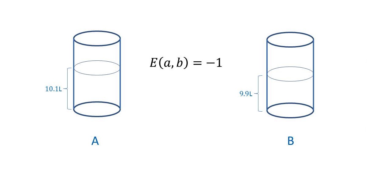
FIGURE \(27.\) Two vessels of over 10L volume each, containing transparent water. The experiment begins with vessel A containing slightly more water, which inevitably leads to vessel B containing less water, which determines the negative expectation value \(E(a,b) = -1\) of the simultaneous quantity measurement.
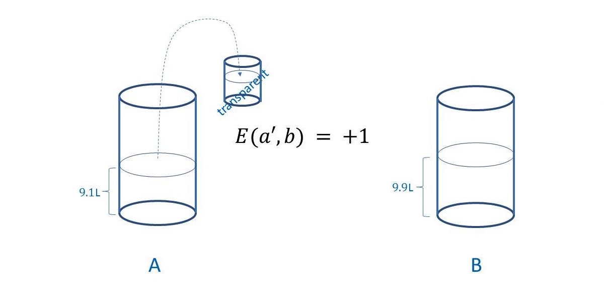
FIGURE \(28.\) The same two vessels of over 10L volume with unequally distributed 20L of transparent water, but this time an aliquot of 1L is taken out from A for transparency measurement, which confirms it. This action ensures the simultaneously carried out quantity measurement on B to be also affirmative. Therefore, we get yes,yes, which results in \(E(a',b) = +1\).
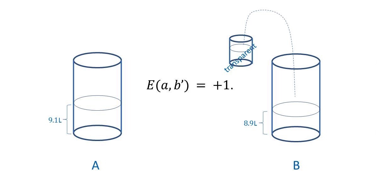
FIGURE \(29.\) Upon the test for transparency on B, by taking a 1L aliquot from it, the picture is reversednow A has more water, and therefore the quantity test on A is affirmative, and, as expected, the transparency test on B is also affirmative. We got yes,yes, as a result of the experiment, therefore its value is \(E(a,b') = +1\).
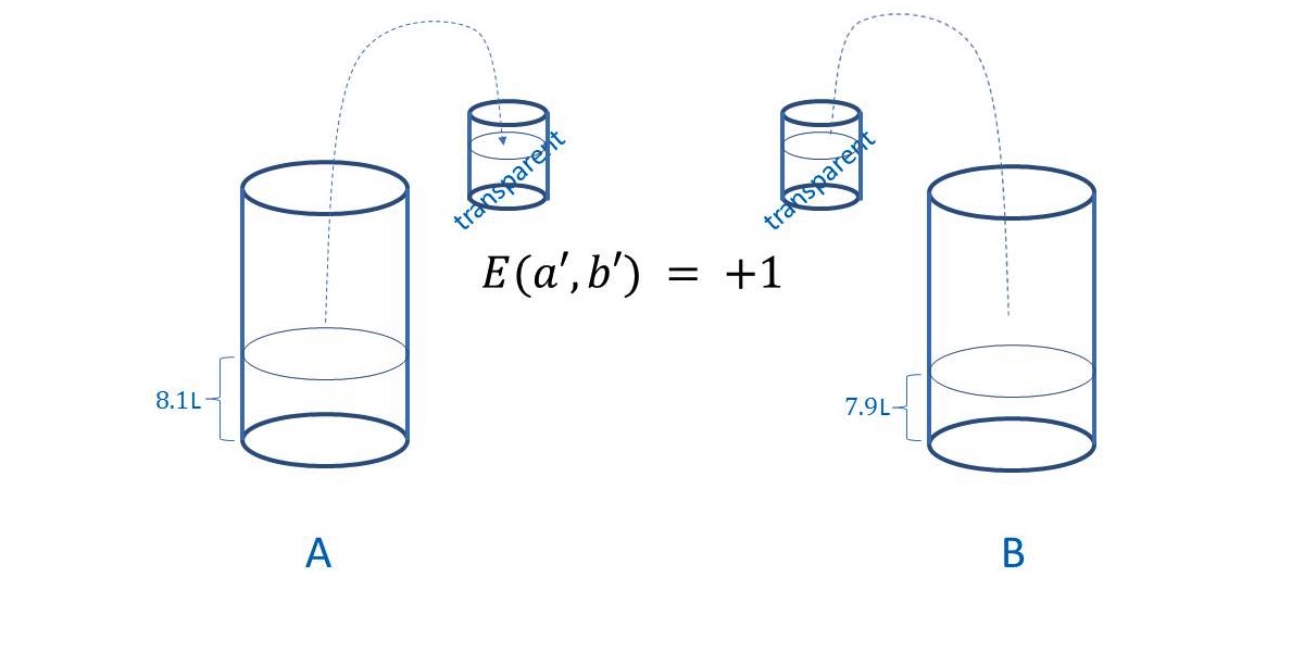
FIGURE \(30.\) This is the easiest experiment. The test for transparency yields an obviously double yes,yes, therefore, the outcome from the experiment is \(E(a',b') = +1\).
We can now sum up the results from all the four experiments\(^{8}\), and plug them into the inequality (4.5) seen on page 179 of ref.\(^{39}\), obtaining \begin{equation}\label{violatedBellsinequality} |E(a,b) - E(a',b)| + |E(a,b') + E(a',b')| = \end{equation} \begin{equation} |-1 - (+1)| + |+1 + 1| = 4 > 2, \end{equation} and the inequality presented in ref.\(^{39}\), an inequality supposedly prone to violation only in quantum mechanics, is violated purely classicallyeq.(\ref{violatedBellsinequality}) shows violation because, according to ref.\(^{39}\) the expression on the left side of the equality must be equal or less than \(2\) if the system behaves classically. If that expression is greater than \(2\), then, allegedly, it is a quantum mechanical system. As seen from eq.(\ref{violatedBellsinequality}), measurements on a purely classical system yield a value \(4\), which is greater than \(2\). Therefore, violation of that inequality cannot be the criterion that a system is not classical but obeys quantum mechanics. We already know, however, that quantum mechanics fails from its very beginnings, therefore the discussed criterion is immaterial anyway.
Now, if someone is wondering why this is the order of plugging into the eq.(\ref{violatedBellsinequality}) of the results from the observations made, it should be noted that it follows the sequence of the measurements seen in FIGURE 27 through FIGURE 30. Besides, there is only one negative unity outcome from the measurements; namely, the outcome \(E(a,b)\). All the other outcomes are \(+1\). Therefore, provided one begins with determining \(E(a,b)\), as one should, any combination of the remaining determinations will result in the same number \(4\) on the left side of the equality.
Both in the here-observed classical case and in quantum mechanical case, the two parts of the system (the two vessels; respectively, the two particles) are not independent of each other from the onset, as a result of the way the problem is construed. The fact that the two vessels, far removed from each other, are not independent (and this is the prerequisite for the violation of the inequalities in ref.\(^{39}\), is not something immediately evident. The dependence between the two vessels is ensured by the initial condition that the total volume of water in the system is 20L. In the same exact way, the fact that the two particles in ref.\(^{30}\) are not independent is not something immediately evident. However, the dependence between these two particles is ensured from the beginningtheir imaginary state is described by a common construct, a \(\psi\)-function, for what it's worth (recall the non-physical and mathematically inconsistent nature of this \(\psi\)-function, to the extent that it should not be the topic of any discussion pertaining to science).
The parallel between the two classical vessels removed from each other at a great distance, and the two particles in ref.\(^{30}\), can continue also when measurements are considered. When what is constructed as a measurement is carried out by a given observable A, for instance, on the first of the two particles in ref.\(^{30}\), all the eigenvalues of the matrix A representing this observable are known a priori, without exception (although the very act of measurement extracts at random only one member of this set of eigenvalues). Thus, when we apply the matrix A on the \(\psi\)-function, common for the two particles, we do not expect to create something that was not there in the first place, i.e. something that was not there by definition. Exactly because of this initial setup of the function (singlet state), when we measure the momentum \(p\) of the first particle and we find, as a result of this measurement that it is up or (+), then the momentum of the second particle must necessarily be \(-p\) or down because because both particles participate in a singlet state, the concrete values of \(p\) being completely random (if we repeat the experiment the concrete value of \(p\) may be different). Furthermore, it should never be forgotten that the most we can speak of in these calculations, is linear algebra, endowed with the idea that it has physical meaning, which is not always the case. To say nothing of the instances, which were discussed earlier, whereby the purported linear algebra does not make sense. This is not to say that there is no mathematical discipline known as linear algebra. However, the way it is used to represent the physical world, is unacceptable, not only because it is non-physical, but because it also violates the elementary requirements of formal logic and reason.
It is to be noticed now, in connection with the above classical experiment, that if we like to wonder at various things, as some groundlessly do in quantum mechanics, we can do it in the case of this classical experiment too. For instance, we may be puzzled by the fact that a measurement \(m(a')\) which we carry out on vessel A and which gives the result yes, that same experiment, in some mysterious way, causes \(m(b)\) to be necessarily yes, not anything else (if someone cares to check that out). Therefore, we may continue, if we consider this path of thought fruitful, that information between A and B has passed at a speed greater than the speed of light, which contradicts the theory of relativity (another question is that the theory of relativity has nothing to do with the speed of information transfer, or with anything at all whatsoever, for that matter. It doesnt, because the theory of relativity is an absurdity, and as an absurdity nothing at all follows from it). We can even write that the common probability \(P(a*b)\) no longer equals the product \(P(a)P(b)\) of the individual probabilities, and conclude all kinds of other things.
It is more reasonable, however, to admit that it is hardly possible to maintain an argument claiming that in all cases whenever there is a connection between two systems, the inequality introduced in ref.\(^{30}\), is violated, and that this violation is entirely plausible, while, on the contrary, in quantum mechanics, an inequality of the sort introduced in ref.\(^{30}\), is violated although there is no connection between the two particles and that makes quantum mechanics something very special. At least, one must reckon with the fact that the entities used to justify violation of the equalities in question, are absurd, as seen earlier in this book.
The above indicates that the notion of two entirely isolated particles in quantum mechanics, somehow exchanging information among themselves, loses content. This is, of course, if we are also not willing to accept (very likely!) that the observed two classical vessels exchange information among themselves.
This discussion is done without assuming the validity of the theory of relativity (cf. here). Not assuming validity of the theory of relativity is undoubtedly the methodologically correct approach (still the more that the theory in question is unequivocally proven to be absurdcf. here). We have especially ignored an often mentioned requirement that the speed of information exchange cannot be infinite. Provided that assumption, probably one may use the above results to even explore the validity of the theory of relativity itself as an exercise in futility (its obvious, unequivocal incorrectness having been shown at once beyond the shadow of a doubtcf. here).
Another strong experimental evidence for the inconsistence of the claims that quantum mechanics describes some special properties characterizing some kind of peculiar micro world, other than the easily accessible for study classical properties of the macro world, are the experiments carried out by Couder\(^{40}\).
A Quantum Mechanical Measurement Leading to Simultaneous Spin-Up and Spin-Down State of a Single Electron\(^{9}\)
This section gives a flare of what contemporary esoteric language of quantum mechanics looks like, hermetically concealing the poverty of physical meaning. This is a demonstration of unpacking under the crust of formulaic receipts, of physical absurdities, even when using elements of correct mathematics.
Let us begin with some well-known background. As is known, the spin operator (the observable representing the spin of the particle) for the first particle in the compound space of the two two-state particles \(\mathbb{C}^2\bigotimes \mathbb{C}^2\) is \begin{equation} \vec{S}_1 = \frac {\hbar} {2} \left( \vec{a} \cdot \vec{\sigma} \right) \otimes \textbf 1 \end{equation} while the same operator for the second particle is \begin{equation} \vec{S}_2 = \textbf 1 \otimes \frac {\hbar} {2} \left( \vec{a} \cdot \vec{\sigma} \right) \end{equation} where \(\textbf 1 = \left( \begin {array}{cc} 1&0\\ 0&1 \end {array} \right)\) is the identity matrix, \(\vec a\) is a unit vector in some general direction and \begin{equation} \tiny \vec {\sigma} = \left( \sigma_1, \sigma_2, \sigma_3 \right) = \left( \left( \begin {array}{cc} 1&0\\ 0&1 \end {array} \right) \left( \begin {array}{cc} 0&-i\\ i&0 \end {array} \right) \left( \begin {array}{cc} 1&0\\ 0&-1 \end {array} \right)\right) \end{equation} is the vector of the Pauli matrices. In other words, to make an operator act on this \(4\)-dimensional space we have to form a direct product of the identity matrix with the vector of the Pauli matrices (the vector of Pauli matrices is the observable representing the spin of the particle in the two-dimensional space). Now, in a usual manner, we will make three simplifications. First we will drop the coefficient \(\frac {\hbar} {2}\) in the expressions of the operatorsthis will not affect our final result. Second, we will observe the vector of the Pauli matrices directed only in z-direction, \(\vec {\sigma_3} = \left( \begin {array}{cc} 1&0\\ 0&-1 \end {array} \right)\). Third, we will carry out the measurement not along just any vector, but along the z-direction. Thus, we may now rewrite the spin-operators in view of this new notation and show them explicitly in a matrix form \begin{equation} \tiny \vec{S}_1 = \vec{\sigma_3}\otimes \textbf 1 = \left( \begin {array}{cc} 1&0\\ 0&-1 \end {array} \right) \otimes \left( \begin {array}{cc} 1&0\\ 0&1 \end {array} \right) = \left( \begin {array}{cccc} 1&0&0&0\\ 0&-1&0&0\\ 0&0&1&0\\ 0&0&0&-1\\ \end {array} \right) \end{equation} and \begin{equation} \tiny \vec{S}_2 = \textbf 1 \otimes \vec{\sigma_3} = \left( \begin {array}{cc} 1&0\\ 0&1 \end {array} \right) \otimes \left( \begin {array}{cc} 1&0\\ 0&-1 \end {array} \right) = \left( \begin {array}{cccc} 1&0&0&0\\ 0&1&0&0\\ 0&0&-1&0\\ 0&0&0&-1\\ \end {array} \right) \end{equation} Obviously, the unit vector along the z-axis is dotted into the above matrices.
The basis states for the direct product of the single electrons, comprising a pair we are to observe are four, namely: \begin{equation} \begin{array}{cc} |++\rangle, |+-\rangle\\ |-+\rangle, |--\rangle \end{array} \end{equation} We will observe one special state in which our two spin--S particles can supposedly exist, namely the so-called singlet state, which under the conditions of our discussion is written as: \begin{equation} |\psi\rangle = \frac {1} {\sqrt{2}} \left( |+-\rangle - |-+\rangle \right) \end{equation} Now, if we are to carry out an experiment to determine the spin of the first particle we have to act on this \(|\psi\rangle\) with the operator \(\vec{S_1}\).
It can be shown that if a measurement is to be performed, there is a 50% chance of obtaining eigenvalue \({S^z_1} = 1\). There is also a 50% chance of obtaining \({S^z_1} = -1\). Suppose now that as a result of the measurement the eigenvalue \({S^z_1} = 1\) was indeed obtained (the probability of \(\left| -\frac {1} {\sqrt{2}} \right|\) 50% was realized). Then the subsequent state of the system would be \(|+-\rangle\), i.e., the \(1^{st}\) electron will be in a spin-up state while the state of the \(2^{nd}\) electron will be spin-down.
The opposite would be the case if as a result of the measurement the obtained eigenvalue were \({S^z_1} = -1\). In such a case, the subsequent state of the system would be \(|-+\rangle\), i.e., the \(1^{st}\) electron will be in a spin-down state while the state of the \(2^{nd}\) electron will be spin-up.
Similar will be the case with the operator \(\vec{{S_2}}\) and its eigenvalues and eigenvectors.
So far this is a well-known state of affairs. Now, however, we want to explore whether the two operators, namely \(\vec{{S_1}}\) and \(\vec{{S_2}}\), can have simultaneously the same set of eigenvectors. As is known, a criterion for two operators to have simultaneous eigenfunctions is their commutator to equal zero. In other words, we have to explore whether the following equality is true: \begin{equation} \left[ \vec{{S_1}},\vec{{S_2}} \right] = \vec{{S_1}}\vec{{S_2}} - \vec{{S_2}},\vec{{S_1}} = 0 \end{equation}
This can be checked immediately: \begin{equation} \tiny \vec{{S_1}}\vec{{S_2}} = \left( \begin {array}{cccc} 1&0&0&0\\ 0&-1&0&0\\ 0&0&1&0\\ 0&0&0&-1\\ \end {array} \right) \left( \begin {array}{cccc} 1&0&0&0\\ 0&1&0&0\\ 0&0&-1&0\\ 0&0&0&-1\\ \end {array} \right) = \left( \begin {array}{cccc} 1&0&0&0\\ 0&-1&0&0\\ 0&0&-1&0\\ 0&0&0&1\\ \end {array} \right) \end{equation} and \begin{equation} \tiny \vec{{S_2}}\vec{{S_1}} = \left( \begin {array}{cccc} 1&0&0&0\\ 0&1&0&0\\ 0&0&-1&0\\ 0&0&0&-1\\ \end {array} \right) \left( \begin {array}{cccc} 1&0&0&0\\ 0&-1&0&0\\ 0&0&1&0\\ 0&0&0&-1\\ \end {array} \right) = \left( \begin {array}{cccc} 1&0&0&0\\ 0&-1&0&0\\ 0&0&-1&0\\ 0&0&0&1\\ \end {array} \right) \end{equation} As can be seen above, the two products are identical, which implies that, indeed, the commutator in question is zero. This, however, means that the operators \(\vec{{S_1}}\) and \(\vec{{S_2}}\) have simultaneous eigenvectors.
However, if that is the case, then the simultaneous application of \(\vec{{S_1}}\) and \(\vec{{S_2}}\) on the state \(|\psi\rangle\) may lead to a situation whereby application of \(\vec{{S_1}}\) will bring about the eigenvector \(|+-\rangle\), while the application of \(\vec{{S_2}}\) will bring about the eigenvector \(|-+\rangle\). This is an algebraically viable situation since the operators \(\vec{{S_1}}\) and \(\vec{{S_2}}\) share these two eigenvectors.
However, this outcome of the measurement will bring about a confusion, from a physical point of view, as to what exactly the subsequent state of the electrons is. For instance, the subsequent state of the \(1^{st}\) electron after the measurement done with \(\vec{{S_1}}\) will be spin-up while the subsequent state of this same \(1^{st}\) electron but as a result of measurement with \(\vec{{S_2}}\) has to be spin-down. Therefore, according to this argument, in 50% of the cases after the measurement, the \(1^{st}\) (and the \(2^{nd}\)) electron will be at once both in spin-up and spin-down state. This outcome of our thought experiment, however, is contrary to the laboratory experimental observations---so far an electron existing simultaneously in spin-up and spin-down state has not been observed experimentally.
One may even argue further that in allowing for the very possibility for both \(1^{st}\) and \(2^{nd}\) particle to be spin-up in a collapsed state; i.e., for the possibility for the subsequent state to be \(|++\rangle\) (respectively, \(|--\rangle\)), we, in fact, allow for the possibility for a state to exist, the probability of whose establishment is \(0\)%. In other words, the two observers cannot make it so that through their measurements the final state will be \(|++\rangle\) (respectively, \(|--\rangle\)). This is an argument which rejects the mere possibility for simultaneous measurement carried out by two observersbecause for such a measurement a situation may be encountered whereby an improbable final state such as \(|++\rangle\) (respectively, \(|--\rangle\)) will be established. However, there is nothing to forbid, as far as a physical experiment is concerned, two experimenters from carrying out simultaneous measurements on this system. In other words, if an observer carries out an independent but simultaneous measurement on the \(2^{nd}\) particle, then according to the above example, that observer may find that the probability of getting spin-up or spin-down may not turn out to be 50%. This will be due to the fact that, unsuspectedly, someone else is carrying out simultaneous measurements on the \(1^{st}\) particle (as mentioned, there is nothing to forbid two independent observers from carrying out measurements on each one particle simultaneously). But not getting 50% probability goes contrary to the result established on the basis of quantum mechanical principles, that the probability must be 50%.
Discussion
Here we will reiterate some of the above and in the process add some more conclusions. For instance, we will note that we discuss a non-degenerate case and will again emphasize the followingthe fact that the operators \(\vec{{S_1}}\) and \(\vec{{S_2}}\) commute is very important to realize because it is the pivotal point of the whole argument. Thus, suppose that we have convinced ourselves that \(\vec{{S_1}}\) and \(\vec{{S_2}}\) indeed commute (as we actually did above). In such a case we do not doubt that these two operators have simultaneous eigenvectorsthis is exactly what the algebra requires. Therefore, nothing prevents us from accepting that, in a case when operator \(\vec{{S_1}}\) has the eigenvector \(|+-\rangle\), operator \(\vec{{S_2}}\) has simultaneously the eigenvector \(|-+\rangle\). Note that even before we spoke about the commutator we had established that \(|+-\rangle\) and \(|-+\rangle\) are eigenvectors of \(\vec{{S_1}}\) and \(\vec{{S_2}}\). Now, however, after we convinced ourselves that the commutator \(\left[ \vec{{S_1}},\vec{{S_2}} \right] = \vec{{S_1}}\vec{{S_2}} - \vec{{S_2}},\vec{{S_1}} = 0\), we already know something more, namely, we now know that these two vectors can be the eigenvectors of the observed operators simultaneously.
Let us imagine further that there are two observers who carry out simultaneously and independently measurements of the spin of the particles. The first observer uses for this purpose operator \(\vec{{S_1}}\) to measure the spin of particle #1. The second observer uses the operator \(\vec{{S_2}}\) to measure the spin of particle #2.
As was shown above, each one of the observers has a 50% chance to prepare the system after the measurement in a subsequent state \(|+-\rangle\) as well as a 50% chance to prepare the system after the measurement in a subsequent state \(|-+\rangle\).
In other words, one possibility is that the first observer has a 50% chance to prepare the system, as a result of the measurement in the state \(|+-\rangle\), while the second observer has the chance to prepare the system, as a result of the measurement, in the state \(|-+\rangle\).
Now notice, since the observers carry out their experiments simultaneously, none of them is in a position to prepare the system in a certain definite state, suitable for a predictable experimental result to be obtained by the other observer. The results of the experiments of both observers will be purely random.
Let us imagine now that out of the several possible results, the two observers happen to realize exactly the result supposed a minute ago; i.e., the first observer turns out to have prepared the system after the measurement in a state \(|+-\rangle\), while the second observer, it turns out, happens to have prepared the system after the measurement in the state \(|-+\rangle\). As already mentioned several times, nothing so far forbids us to suppose such a possibility: \(|+-\rangle\) and \(|-+\rangle\) are eigenvectors both of \(\vec{{S_1}}\) and of \(\vec{{S_2}}\). \(\vec{{S_1}}\) and \(\vec{{S_2}}\) commute, therefore the eigenvectors in question can be observed simultaneously, the observers carry out their experiments on the virgin, if I may say so, function of state \(|\psi\rangle\) (i.e. there is no reason to suppose that the mentioned 50-50 chance is not valid any more). Therefore, so far everything is in accordance with the formal requirements of quantum mechanics and, according to the rules of quantum mechanics, nothing formally, from the point of view of linear algebra, forbids us to obtain the mentioned result. However, if it turns out that there are problems with the physical interpretation of the above-obtained result, although obtained in full compliance with the quantum mechanical rules, then these problems would put under question the quantum mechanics theory of measurement itselfa theory which leads to a non-physical result is an incorrect theory. Unfortunately, even a superficial glance at the result we obtained abovea system existing after the measurement both in state \(|+-\rangle\) and in state \(|-+\rangle\)shows that there are indeed problems. Thus, as already mentioned, there is a chance, as a result of the quantum mechanical experiment, for the spin of particle #1 to be both spin-up and spin-down (same applies to particle #2). Such a result, however, obtained on the basis of quantum mechanics prescriptions, is not in accordance with the well-established experimental facts in the laboratorya state of the particle (e.g. an electron), in which this particle has both spin-up and spin-down, has never been observed experimentally. Conclusionquantum mechanics experiment, conducted in full concordance with the rules of quantum mechanics, has led to an outcome that does not have physical meaning. It is not uncommon in science. when physical inconsistency of even such a seemingly insignificant level is found, to cause reconsidering the rules of a theory, even a theory of the magnitude of quantum mechanics, even its collapse. We have seen already from the previous arguments in this book, that, unfortunately, in the case of quantum mechanics theory, the latter outcome is the valid one.
Here is a brief recount of the above. We determine that two operators are commuting. The fact that these operators are commuting means that they have simultaneous eigenvectors, even if these eigenvectors are orthogonal. Thus, algebraically, we can choose any combination of these eigenvectors, and still the eigenvectors comprising the couple will remain simultaneous. Surprisingly, however, it turns out that if we want this outcome to have physical meaning, the discussed simultaneity is not always acceptable. When the two operators act on one particular state vector (singlet state), two of the common eigenvectors, for purely physical reasons, cannot be simultaneous. It turns out that for physical reasons, specifically, orthogonal eigenvectors cannot be simultaneous, despite the fact that, algebraically, there is no requirement that the two eigenvectors of these two commuting operators should not be orthogonal, for these vectors to be simultaneous eigenvectors.
Thus, notice the contradictionaccording to the commutativity of \(\vec{{S_1}}\) and \(\vec{{S_2}}\), algebraically, there is certainly a 50% chance to observe simultaneously the vectors \(|+-\rangle\) and \(|-+\rangle\). However, according to the paradoxicality of such an outcome, the simultaneous obtainment of these vectors is impossible from a physical point of view.
Thus,
the two observers may prepare the system simultaneously in the states
\(|++\rangle\) and \(|++\rangle\)
\(|--\rangle\) and \(|--\rangle\)
\(|+-\rangle\) and \(|+-\rangle\)
\(|-+\rangle\) and \(|-+\rangle\)
but they
also can prepare it in the physically impossible states
\(|+-\rangle\) and \(|-+\rangle\)
\(|-+\rangle\) and \(|+-\rangle\)
\(|++\rangle\) and \(|--\rangle\)
\(|--\rangle\) and \(|++\rangle\)
This is easy to understand, when realizing that the first sign within the shell \(|spin \ of \ first \ electron \ \ \ \ spin \ of \ second \ electron\rangle\) concerns the first electron, while the second sign concerns the second electron, and that (+) is for spin-up, while (-) is for spin-down. Thus, it is seen that in 50\(\%\) of the cases the first electron, respectively, the second electron, is prepared simultaneously in spin-up and spin-down state, which is physically impossible.
Thus, algebraically, the simultaneity of two eigenvectors of two commuting operators, is undeniable. The physical impossibility for the last two couples of eigenvectors to exist simultaneously is only due to the fact that they emerge from a construct (singlet state) which is proposed to be a viable physical entity but is not. As seen, such a formal proposal breaks down physically under the conditions of a simultaneous measurement discussed above.
If the above considerations are acceptable and we have to exclude the singlet states as viable physical entities, then a concept such as non-locality, which is a direct result of improperly considering the singlet state as physically viable, also has to be abandoned since its physical meaning will be questionable as well.
In other words it is not that non-locality is some kind of property of quantum mechanics, which we have to take for granted, and which gives rise to phenomena worth discussing. Quite the opposite, the notion of non-locality is a consequence of the standard formal acceptance in quantum mechanics that even strange entities such as singlet state, as long as they are products of the Hilbert space, are physically realizable. As we saw above, from physical point of view, the reality of such a state is, in fact, problematic.
Of course, as critical such conclusion is on its own, we can make it only if we consider quantum mechanics a legitimate field of scientific study, bringing sensible topics for discussion. However, as we saw from the arguments presented herewith, quantum mechanics is an illogical, inconsistent endeavor in its fundamentals, an endeavor which has no place as a topic of scientific exploration, neither of any discourse that might accompany it.
Physical Molecule
As explained here, this book does not discuss experiments, especially such claiming confirmation of quantum mechanics effects, much less does it discuss experiments, connected with relativity. Relativity is an absurdity, and therefore there never can be anything, least of all an experiment contemplated, remotely connected to relativity. The same applies to experiments claimed to confirm the reality of quantum mechanics. There can be none. Quantum mechanics, however, is name-dropped every time some research or an esoteric statement is meant to sound important and high-browed. In view of what was said in this book, such uncalled-for enthusiasm must be discouraged, with very few exceptions, which, although adorning themselves with quantum mechanical lingo, may have importance for a completely different reason. Thus, one may inspect a curious experiment, which was performed, claimed to be based on the so-called quantum tunneling, although what it really comprises is processing a signal from a very clever technical contraption. I encountered this study during my work on phase formation\(^{41-43}\) and shared my finding with C. I. Noninski, knowing about his fundamental work on phase formation, which predicted the behavior reported in the study in question\(^{44,45}\). My father expressed a keen interest and we worked together on the study reported below. We wrote an account of this work and submitted it for publication but the reviewer required that he should be put as a co-author of the study, in order to give it a favorable review, which we refused to do and the paper was not published.
This is an example of something useful for other reasons that may come out, despite no apparent connection to a subject considered modernquantum mechanics. Although the authors spruce it up by a claimed quantum effect, the so-called quantum tunneling, is in name only.
The following is also an illustration, showing that important, fundamental matters in science need not be flabbergasting in their appearance and impenetrable in their math. Very deep understanding of matter can be achieved by simple means.
How substances are built has been of continued interest in physics, the general understanding being that individual atoms or molecules, rather than clusters, form the structures of substances in their thermodynamically stable state. Contrary to this understanding, existence of thermodynamically stable atomic and molecular formations (clusters)droplets and small crystalshas been established for the first time by C. I. Noninski\(^{46,47}\) and later on studied also by this author in refs.\(^{41-43}\), based on the Gibbs-Thomson isotherm, corrected for the dependence of surface tension on the radius of the droplet (small crystal).
Here\(^{83}\), definitive evidence is shown that formations seen in Binnig and Rohrer\(^{44,45}\) are not individual Si ad-atoms, as the authors claim, but are clusters of Si atoms, as are the C clusters in Kroto et al\(^{48}\), but consist of less than 60 C atoms, in opposition to the current belief.
These findings further our understanding concerning the buildup of substances.
Below, analysis of experimental stable clusters is carried out, avoiding the use of models. The reliance on firmly established undeniable facts is undertaken in order to preempt any possible objections or speculations.
The scanning tunneling microscope (STM) provides a unique possibility, unmatched by any other technique, to measure exactly the real size of objects of molecular and atomic dimensions, carrying out such measurement directly, not through comparison with calibration standards, as required for the Scanning Electron Microscope (SEM).
The maxima in FIGURE 31, observed with STM on the reconstructed Si (111) surface are interpreted as Si atoms sitting on top of the Si (111) surface, in distinct sites and arranged in a unique manner. However, closer inspection of the data presented in refs.\(^{44,45}\) reveals otherwise.
Thus,
observe carefully where the long diagonal under discussion is
situated, lying between the first and the second deep minimadrawn
here by a white vertical line in FIGURE
31. The number of maxima comprising the 7 x 7 unit cell are 12,
including the 4 maxima lying on the long diagonal. The surrounding 9
minima (3 deep and 6 shallow) around the triangular 6-maxima
formations, are also seen.
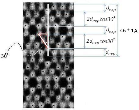
FIGURE \(31.\) Top view of the original shining example of an STM graph presented in Fig. 5 of ref.\(^{44}\) and in Fig. 1 of ref.\(^{45}\) of the relief of two complete 7 x 7 cells, taken at 300\(^{o}\)C. Long and short diagonals are \(46 \pm 1 \overset{\circ}{\text{A}} \) and \(29 \pm 1 \overset{\circ}{\text{A}} \), respectively. The 30\(^{\circ}\) angle follows from the short cathetus facing that angle being \(\frac{1}{2}\) of the hypotenuseobserve the three maxima forming the hypotenuse and the two maxima forming the short cathetus.
The
mentioned 4 maxima, which lie on the long diagonal, divide it into the
following 5 parts:
?
One part, situated at its middle, whose length is equal to
\(d_{exp}\).
?
Two parts at its ends, comprising the distance between the deep minima
and maxima neighboring them with one and the same length, equal to
\(d_{exp}\).
and
?
Two more parts, each one is of length equal to
\(2d_{exp}cos30^{\circ}\),
from where, having in mind that the authors have measured the long diagonal to be \(46 \pm 1\overset{\circ}{\text{A}} \), the value of the quantity \(d_{exp}\) can be calculated; namely, the diameter of each formation, appearing as a maximum on the Si surface: \begin{equation} 3d_{exp} + 4d_{exp}cos30^{\circ} = 46 \pm 1 \overset{\circ}{\text{A}} \end{equation} and, therefore \begin{equation}\label{dexpSi} d_{exp} = 7.12 \pm 0.15\overset{\circ}{\text{A}}, \end{equation} which gives for the value of the Si cluster volume the following: \begin{equation}\label{vexp} v_{exp} = \frac{4}{3} \pi \left( \frac{d_{exp}}{2} \right)^3 \approx 189{\overset{\circ}{\text{A}}}^3. \end{equation} To see how this value compares to the volume of a single Si atom, divide the density of Si by its atomic weight to obtain the number of moles of Si in \(1cm^3\) and then multiply that quotient by Avogadro's number to get the number of atoms in \(1cm^3\). The inverse of the obtained result is the volume \(v_{_{_{Si}}}\) occupied by one Si atom: \begin{equation}\label{20} v_{_{_{Si}}} = \frac {{A_{_{Si}}} } {\rho_{_{Si}}N} \approx 20\overset{\circ}{\text{A}}^3, \end{equation} where \(A_{Si} = 28.085g \ mol^{-1}\) is the atomic weight of Si, \(\rho_{Si} = 2.3290g \ cm^{-3}\) is the Si density and \(N = 6.022 \times 10^{23}mol^{-1}\) is Avogadros number.
From the above, it is obvious that the value \(v_{exp}\) of the formations seen in FIGURE 31 is not the volume of a single Si atom \(v_{_{_{Si}}}\), calculated from the known data, but is almost 9.5 times greater.
In another example, whereby the volume \(v_{_{_{C}}}\) of one single C atom is \begin{equation}\label{8.86} v_{_{_{C}}} = \frac {A_{_{C}}} {\rho_{_{C}}N} \approx 9\overset{\circ}{\text{A}}^3, \end{equation} where \(A_{_{_{C}}} = 12.0107g \ mol^{-1}\) is the atomic weight of C and \(\rho_{_{_{C}}} = 2.25g \ cm^{-3}\) is the density of C, ref.\(^{48}\) reports the value \(d_{exp} \sim7\overset{\circ}{\text{A}} \) for the diameter of C cluster (note the similarity of this value with \(d_{exp}\) of Si, eq.(\ref{dexpSi})). Therefore the volume of the C cluster is \(\sim 180\overset{\circ}{\text{A}}^3\), as calculated from eq.(\ref{vexp}), which is about 20 times greater than the volume of a single C atom and is not 60 times as great as the authors of ref.\(^{48}\) claim.
This study only deals with indisputable experimental facts. Therefore, it will not discuss the theoretical reasons why a monolayer of clusters is thermodynamically more stable than a monolayer built of separate atoms or molecules, or why it may be expected that the formation of the clusters occurs due to the limited effective radius of action of the intermolecular forces\(^{47}\), reached at the critical temperature, the same factor that leads to absolute boiling, whereby the surface tension of any droplet (small crystal) of the substance, independently of its radius, will become equal to zero. In addition, here only the experimental fact\(^{49}\) is noted that the quotient \(\frac{\rho}{\rho_c} = \frac{\rho MN}{\ rho_cMN} = \frac{v_c}{v} \approx 3\), where \(\rho_c\) is the critical density, \(\rho\) is the density at a temperature much lower than the critical temperature, \(M\) is the molecular weight and \(v_c\) is the critical molar volume, and it is observed that this quotient's value does not depend on the nature of the substance. The \(\frac{\rho}{\rho_c}\) ratio has the slightly higher value of about 4.5 for the available (estimated) data of all studied metals, which may be underestimated in view of the above-discussed experimental results, especially those of refs.\(^{44,45}\)
\( \LARGE \mathbb{FOR \ QUANTUM \ MECHANICS \ TO \ TAKE} \)
DIRECTIONS FOR REPLACING QUANTUM MECHANICS BY DEVELOPMENTS IN CLASSICAL MECHANICS
The facts shown, concerning the governing doctrines in contemporary science, prove that the basics of fundamental science are crying out loudly for a major overhaul. In the first place, science must part entirely with the theory of relativity. Every bit of it must go, and we need not say a word more about it.
As for quantum mechanics, it must return to its classical mechanics roots. Below, we will direct our attention to some developments, which were begun by C. I. Noninski, his spirit hanging over the whole section, to which I have contributed my own input as well.
I would like to give full credit to C. I. Noninski, who has initiated me into thinking about these issues at all. Thus, although unpublished, and, although I have developed some of these ideas in a major way, the basis of the ruminations in this book about the three laws of Newton as being laws of rest, as well as the necessary expansion of the second law (here), action in classical physics (cf. here), violation of the principle of least action (cf. here), action when a body moves between two positions of rest (cf. here), and classical uncertainty principle (cf. here), are entirely his ideas, which he has shared with me.
Of course, when speaking about contributions, the discovery that \(v^2 = 2ax\) is the most fundamental absolute relation of mechanics, when it comes to real, operative motion\(^{84}\) of a free body under the effect of a constant force and all the conclusions therefrom, especially the fact that the expanded Newton second law \(F_{real} = ma + \frac{mv^2}{2x}\) is an absolute equality, arriving from \(v^2 = 2ax\) before any other discovery in physics, including Newtons second law, are entirely mine [VCN] (cf. here). Connected with that discovery, albeit not connected with the operational character of motion, but concerning Galileos discovery of the non-operational essence of uniform translatory motion, is the contribution, entirely mine, revealing the catastrophic absurdity of relativity, due to the application of the non-physical, as well as mathematically inconsistent, Lorentz transformations. This discovery has led me to further unequivocally discover the absoluteness of time and spacethe greatest discovery ever made in science, because it concerns the most fundamental notions of science and of thinking in general. Furthermore, the combination of my unequivocal discovery that relativity is absurdity, on the one hand, and on the other, that \(v^2 = 2ax\) is the ultimate absolute equality in mechanics, led me to the conclusion that it is not Newtonian physics that is to be considered as the most fundamental grounds of physics, but what must be treated as such, is the absolute character of the fundamentals of physics, such as its definitions, surprisingly, obviously neglected in their full sense. A curious accompanying fact to that finding, is my discovery that the mass-energy relationship \(E = mc^2\), which the absurd theory of relativity cannot derive despite the frantic propaganda that it does, is inherent in the very fundamentals of classical physics, these fundamentals existing prior to any other discovery in physics, including the discoveries of Galileo and Newton (here). These fundamentals, which are absolute truths of physics, and which my discovery concerning \(E = mc^2\) arrives from, are the very definitions of basic quantities such as velocity and acceleration.
Another contribution, which I have personally made, is the discovery of the flawed nature of the physical (cf. here) and mathematical (cf. here) basis of quantum mechanics, as well as the fact that, starting from Planck, there are a number of further failed attempts to derive the famous formula for the spectral energy emission density of blackbody radiation.
In this context, one must prominently recognize the seminal work\(^{11}\) of C. I. Noninski, a facsimile of which is shown here.
This is only the beginning of what must become a full-blown effort to replace what is now know as quantum mechanics, by truly scientific endeavors, aimed at furthering the only sensible understanding of the worldthe classical science, science without relativity and quantum mechanics.
Motion
When one looks at science from a birds eye view, even when ignoring the absurd twentieth century physics, based on relativity and quantum mechanics, one finds a notion which stands out as the beginning of the age-long confusion, actually, at the bottom of that confusion, whose unraveling couldn't be more urgent. This notion is motion.
The deeper meaning of motion has been the subject of rumination in philosophical texts, where it has been pointed out that motion is not just a mere repositioning in space, neither is it just a compilation of individual states of rest, but is connected with deeper qualitative changes, such as change in energy, taking place while the body is moving.
Unfortunately, this deeper meaning of motion, with its far-reaching consequences for physics, has not migrated into the standard understanding of classical mechanics. Thus, the idea of motion held by the mainstream, still goes along with the idea, following from the equations used by Newton and Maxwell, that motion is presence of a body at a given moment in a given place, while at another, follow-up moment, the body finds itself in another place. This limited understanding of motion has caused and is causing serious conceptual problems in physics. It has led to the wrong impression that some new physics is due to be developed, that would bring the needed clarification.
C. I. Noninski had started an effort\(^{50,51}\) to clothe that correct understanding of motion in the language of standard classical physics (physics without quantum mechanics and theory of relativity), which would allow science to deal away with its departure from the scientific path it is supposed to followthe path of being the assembler and keeper of veridical, uncorrupted knowledge, free of absurdities and deception. Sadly, for various reasons, C. I. Noninski had not been able to bring the essence of his ideas to a wider audience. This book, which is also based on my extensive discussions with him at the time, is devoted to presenting and developing these sorely needed concepts. Further, ruminating over these past discussions with C. I. Noninski, I came to realize that what has been overlooked in physics, rests in some of the most obvious and fundamental definitions, which are indisputable absolute truths, such as the definitions of velocity and acceleration. A specific contribution of this author, is the realization that the well-known relation \(v^2 = 2ax\), which usually rests in the background, primarily as a student exercise, is in fact the most fundamental equation of mechanics, having dramatic far-reaching consequences, when it comes to characterizing and understanding the motion of a free body impelled by a constant force. As seen here and on, that equation indeed follows from absolute truths in physics, such as, none other, than the definitions of velocity and acceleration; that is, where physics itself begins. Therefore, as said, the absoluteness of \(v^2 = 2ax\) cannot be disputed on any grounds. The parabola in question not only helps understand that the current consideration of the second law and the third law of Newton as laws of motion contradicts Newtons first law, but also, when undergoing inevitable expansion, inherently contains the uncertainty principle (to be discussed latercf. here), thus far attributed only to quantum mechanics. Therefore, although known formally, the true, deeper significance of the expression \(v^2 = 2ax\) for physics has not been recognized to date.
It
is not unusual in physics to have far-reaching conclusions based on
some seemingly simple and trivial observations. A telling example in
that respect is the second law of thermodynamics, which has
many formulations. Even the apparently most involved of these
formulations ultimately reduces to this simple statement:
Transfer
of heat cannot occur spontaneously from a colder to a warmer body.
The above formulation, although, as mentioned, seemingly simple, has such ramifications, that it can truly be considered as the backbone of all contemporary science. I remember wondering from my first days in science, how such simple, everyday observation, could be the basis of all science, but it is.
In
a similar fashion, the very fundamentals of physics can be shaken, as
will be seen, when not refusing to consider (as physics has done until
now) the obvious fact that
motion, across a non-zero spatial distance \(\Delta x\), of a free body of mass \(m\), acted upon by a constant force, will inevitably be accompanied by a change in its velocity.
\(^{85}\)No axioms or postulates prone to discussion are involved in the above absolute law, only the absolute truths of physics. Curiously, the above velocity requirement is to be satisfied by the most common formulae physics uses at large. Alas, that requirement has not been recognized, despite its absolute character. Hence, neither has it been explicitly present in the expressions of the laws used by the mainstream.
Before
proceeding with the main argument, it may be noted that in ruminating
about the above absolute law; namely, that change of velocity is
mandatory when a body undergoes a real spatial shift \(\Delta x\), one
may put forth the following argument: although, by the very definition
of the term velocity \(\left( v = \frac {\Delta x} {\Delta t}
\right)\), the traveling through a real distance \(\Delta x \ne 0\)
cannot occur at velocity \(v = 0\), it may wrongly appear that if the
motion is linear and uniform (alternatively, we call such
motion uniform translatory motion), whereby velocity \(v\) is
not zero, such traversing of a distance \(\Delta x\) at a constant
velocity \(v = const\), is a common mode of motion. Recalling from herequite
significantly and emphatically, however,
\[ \bbox[5px, border: 2px solid grey]{ uniform \ translatory \
motion, \ is \ akin \ to \ rest.} \nonumber \]
Galileo discovered this phenomenon some 400 years ago, correcting the prevailing Aristotelian view that all motion is operative. Uniform translatory motion is not operative, despite the word motion in its name. Later, at the beginning of the twentieth century, the principle of relativity, consisting of the fact that the uniform translatory motion is akin to rest, discovered by Galileo, was badly botched, creating one of the most shameful blunders in human history (cf. here), causing mass degradation of societies through acquiring wide social penetration.
In connection with the above, it must be noted, that the discussion and the derivations herewith concern the motion of a free body acted upon by a constant force, while the mentioned uniform rectilinear motion of a body, not acted upon by a constant force, is not the subject of discussion in this section of the book.
We
should, nevertheless, mention that some laws of classical mechanics
said to be laws of motion, such as Newtons first law of motion (law
of inertia)
Every
object persists in its state of rest or uniform linear motion,
unless it is compelled to change that state by an unbalanced force
impressed on it
are valid with theoretical exactness only in the case of uniform linear (translatory) motion. In fact, motion is overcoming of Newtons third law, in a sense, its negation, so that Newtons first law, ensuring rest, would no longer be in effect.
Accidentally, and that needs repeating here and will be backed by more evidence later (Hamiltons equations) , Newtons third law, the law of equality and oppositeness of action and reaction, and its application, Newtons second law, the latter expressed as \(F = ma\), would be in contradiction with the above-quoted Newtons first law, if these laws are referred to as laws of motion. Newtons three laws are, rather, laws of rest.
To correct this and have force reflect real motion, what follows next is an inevitable expansion, denoted by \(F_{real}\), of the notion of force described by Newtons second law.
Newtons Second Law and Velocity Change During Real Spatial Shift Caused by Constant Force
The derivations which follow, use the definitions put forth here.
As mentioned above, uniform translatory motion is impossible in a force field where motion impelled by an uncompensated force, is inevitably connected with acceleration (change of velocity with time) governed by the operative, non-compensated part of the expanded Newtons second law; that is, the part, seemingly of the same appearance as the known Newton second law: \begin{equation} \label{Newtonssecondlaw} F = ma, \end{equation} where \(F\) is half of the real force \(F_{real}\) (why this is so will be seen below). Eq.(\ref{Newtonssecondlaw}) comprises the non-compensated part of \(F_{real}\), applied on a body of mass \(m\), and causing acceleration \(a\).
We are getting ahead of ourselves here, regarding a central question which will be revealed later. In a word, if this is not too confusing at this point, it may only be added that the above eq.(\ref{Newtonssecondlaw}) only has the appearance of the known Newton second law, but, as will be seen, it has a different, operative, physical meaning. When the expanded Newton second law is involved; that is, when there is acceleration, we speak about genuine motionthis is motion in its true, operative sense.
Further,
it may appear that Newtons second law, when written as
in eq.(\ref{Newtonssecondlaw}), having the well-known outer appearance
of that law, completely describes force \(F\) applied to a body of
mass \(m\). In particular, it may appear that, because of the presence
of \(a = \frac {v} {t}\), which is accounting for the velocity \(v\)
of the body, while the point of application of \(F\) is transported
across a displacement \(x\), there is work \(A\) produced in the
process, namely, \begin{equation} A = F x = ma \, x. \end{equation}
However, it cannot be farther from the truth to assert that
eq.(\ref{Newtonssecondlaw}), if perceived as Newtons second law in
its known form, describes motion completely. This can be seen by
considering Newtons third law
For
every action, there is an equal and opposite reaction
or
expressed in terms of force:
Whenever
a first body exerts a force F on a second body, the second body
reacts by exerting a force -F on the first body. F and -F are equal
in magnitude and opposite in direction.
Whereby, if \(F = ma\), in a sense well-known in the standard literature, were the only force causing the displacement \(\Delta x\), then adding to it the equal and opposite inertial force \(F^* = -ma\), required by the above-mentioned known Newton second law, will yield as a result \begin{equation} \label{} F - F^* = ma - ma = 0. \end{equation} When to \(F\), its reaction \(F^*\), naturally arising as Newtons third law prescribes, is added, with a negative sign, then it must inevitably follow that transporting the body through a distance \(\Delta x \ne 0\) has been achieved without doing any work \(A\) \begin{equation} \label{Work} A = (F - ma) x = 0. \end{equation} Equation (\ref{Work}), which is usually referred to as DAlemberts principle, when the displacement is a virtual displacement \(\delta x\), is paradoxical when the displacement \(x\) is real. This paradoxical equation, expressing the possibility to have real displacement without doing work, comes about, if we accept that the only effect of the force \(F\) on the body is to cause the appearance of the counteracting force \(F^*\) alone, and nothing else, such as, causing, for example, change of velocity of the body. In other words, eq.(\ref{Work}) implies that the velocity \(v\) of the body at the beginning of the displacement \(x\) (denoting \(\Delta x\) as adopted here, is the same as the velocity \(v\) of the body at the end of that displacement. If that were the case, however, it would mean that the observed motion is not a uniformly accelerated motion under the action of a constant force \(F\), as it really is, but is uniform translatory motion, akin to rest, which is not the case when a constant force acts on a free body.
Therefore, because of the very essence of the motion of a free body acted upon by a constant force, that constant force should be \(F_{real} > F\) and its effect on the body is not only the creation of an inertial counter force \(F^* = -ma\) but is also causing a change in the velocity of the body from velocity \(v_{0}\), say \(v_{0} = 0\), at the beginning of the displacement \(x = 0\), to velocity \(v_{1} \ne v_{0}\) at the end of that displacement; which is nothing other than causing the body to acquire kinetic energy \(\frac {mv^2} {2}\) at the end of the displacement \(x\): \begin{equation} \label{correctedDAlembert} A = (F_{real} - ma) x = \frac {mv^2} {2}. \end{equation} Thus, the whole expression for the force \(F_{real}\), acting on the body, which causes motion; that is, causing the real spatial shift \(\Delta x\) along with changing velocity \(v\) of the body, is \begin{equation} \label{FIRSTOCCURRENCEOFrealforce} F_{real} = ma + \frac{mv^2}{2 x}. \end{equation} Notice the second term after the equality sign, the term \(\frac{mv^2}{2 x}\). It expresses energy \(\frac{mv^2}{2}\) per unit displacement \(x\) in space; namely, \(\frac{\frac{mv^2}{2}}{x}\). This linear energy density, is the spatial effect of force.
Conversely, the expression \(F = ma\) of the force, retaining only the first term on the right of eq.(\ref{FIRSTOCCURRENCEOFrealforce}), the way it is present in the standard literature and is known as Newtons second law, is an equation of rest. It reflects only the temporal characteristic of force; namely, the change of momentum per unit time, \(ma\) expressed here as \(\frac{m \Delta v}{\Delta t}\), leaving out the spatial characteristic.
First way to derive the important equality \(ma = \frac {mv^2} {2 x}\)
Now, regarding \(F_{real} = ma + \frac{mv^2}{2 x}\), eq.(\ref{FIRSTOCCURRENCEOFrealforce}), observe the following. Consider the effect on a body of a given force \(F\) in time, (consider the impulse\(^{86}\)) \begin{equation}\label{Ftmv} F t = m v. \end{equation} On the other hand, suppose that there is a real spatial displacement \(\Delta x\) when considering that same force \(F\) as in eq.(\ref{Ftmv}), to be causing that displacement. In such a case, the product \(Fx\), which is work (spent energy), is the effect \(in space\) of that same force \begin{equation*} F x = \frac {mv^2} {2}. \end{equation*} As seen, expressing the effect of that given force \(F\) in those two ways (\(F = \frac {m v} { t} = ma \ \text{and} \ F = \frac {mv^2} {2 x}\)) leads to \begin{equation} \label{forcecomponentequality} ma = \frac {mv^2} {2 x}. \end{equation} From eq.(\ref{FIRSTOCCURRENCEOFrealforce}) and eq.(\ref{forcecomponentequality}) we have \begin{equation} \label{F12Freal} F = \frac{1}{2} F_{real}. \end{equation} And, of course, from eq.(\ref{FIRSTOCCURRENCEOFrealforce}) and eq.(\ref{forcecomponentequality}) it is immediately seen that \begin{equation}\label{twomaFIRSTOCCURRENCE} F_{real} = 2ma \end{equation} and \begin{equation}\label{mvsquaredoverxFIRSTOCCURRENCE} F_{real} = \frac{mv^2}{x}. \end{equation} These three equivalent equations eq.(\ref{FIRSTOCCURRENCEOFrealforce}), eq.(\ref{twomaFIRSTOCCURRENCE}) and eq.(\ref{mvsquaredoverxFIRSTOCCURRENCE}) we will repeat later, especially after proving their validity in an absolute way.
Aside from talking about the above extension of Newtons second law, we should again emphasize the fact that the usual writing of the force equation in the form of \(F = ma\), eq.(\ref{Newtonssecondlaw}), only expresses the effect of the force in time, reflecting its impulse \(F t = m v\), while ignoring the effect of the force in space, along the displacement. Considering the effect of force \(F\) in such a limited way, that is, its effect only in time (or its effect only in space, for that matter), has its clear practical applications when the effect with those limitations is what is required. This practical applicability of \(F = ma\) is the reason why that limited formula is the widely known formula for the force. However, observing the result of application of \(F\) only in time limits the more general conclusions which can be drawn from classical mechanics if the effect of force is observed in its entirety (both in time and in space), as will be seen in a most astonishing way here.
Zenos Aporias
Classical mechanics, observed in the limited fashion, exemplified by the usual expression \(F = ma\) of Newtons second law, resembles the one-sidedness, comprising the sophism of Zenos aporias. Take, for instance, the paradox relating the competition between Achiles and the tortoise. It is true that for Achiles to catch up with the tortoise and even overrun it, he must first travel half the distance separating them, and to travel that half, he must first travel half of that half, and so on and so forth, ad infinitum. Therefore, if the question were as to whether Achiles has to cross half of the distance to the turtle, before catching up with it, we have the answer we need. This is not, however, the answer to the question as to whether or not Achiles can catch up with the tortoise and overrun it, not only because it is not true that passing of a given distance occurs because of passing of a distance, but also because there is not only distance between Achiles and the tortoise, but they also travel a given distance for a certain time, which differs for each one of them. For a given time Achiles travels longer distance compared to the tortoise, Achiles runs at a greater velocity than the tortoiseAchiles will run across a given half a distance for a shorter time than the tortoise would run across that same half a distance. In other words, when such competition is discussed, it is not only distance that matters but also time. Therefore, Achiles will arrive first at the finish, unless the tortoise is so close to the finish line when the competition begins, Achiles lagging behind, that even the high velocity at which Achiles runs, will not be enough to catch up with the inching tortoise, which happens to be due to cross only an insignificant distance to the finish line.
Absolute proof that the expanded Newton second law \(F_{real} = ma + \frac {mv^2} {2 x}\) is an absolute equality
In this section, we will take the opportunity to disperse any doubts regarding the unexpected expansion of Newtons second law, demonstrating, in addition, that it is an absolute law.
When it comes to a free body impelled by a constant force, the standard form of Newtons second law \(F = ma\) is so entrenched in the conscience of those who deal with science, that it seems unbelievable that \(F = ma\) describes force only in a limited sense, only concerning its temporal side, and that it is at all possible that there can be any other equation, expressing the full meaning of force; that is, that there can be an expanded form \begin{equation} F_{real} = ma + \frac {mv^2} {2 x}, \end{equation} eq.(\ref{FIRSTOCCURRENCEOFrealforce}), of Newtons second law, which has also two equivalent variants of expression, respectively, \begin{equation} F_{real} = 2ma, \end{equation} eq.(\ref{twomaFIRSTOCCURRENCE}), and \begin{equation} F_{real} = \frac{mv^2}{x}, \end{equation} eq.(\ref{mvsquaredoverxFIRSTOCCURRENCE}). The doubt that the traditional form of Newtons second law \(F = ma\) describes force in only a limited sense (describes only the temporal part of force), can be removed by demonstrating that the equivalent equations \(F_{real} = 2ma\), eq.(\ref{twomaFIRSTOCCURRENCE}), respectively, \(F_{real} = \frac{mv^2}{x}\), eq.(\ref{mvsquaredoverxFIRSTOCCURRENCE}) of the equation \(F_{real} = ma + \frac {mv^2} {2 \Delta x}\), eq.(\ref{FIRSTOCCURRENCEOFrealforce}), all three causing controversy, can be rearranged into a form, which will be seen to coincide with the rearranged absolute equality \(v^2 = 2ax\), arrived at from absolute truths of physics. This will be an unequivocal proof that these three equivalent forms are correct and inevitable, intrinsic to physics. In fact, these three equivalent forms are the true equations of motion.
Now, we will show this not by employing the violation of DAlemberts principle, as we did when deriving \(F_{real} = ma + \frac {mv^2} {2 \Delta x}\) here, but from the very first principles of physics, embodied by the equation \(v^2 = 2ax\), whose truthfulness is fundamental and which existed before any other discovery in physics.
Thus, begin by preparing the absolute equality \(v^2 = 2ax\), arrived at from absolute truths of physics, in a form suitable for comparisonin this analysis we need to know the absolute expression of momentum, \(p = mv\), which arrives from the absolute expression \(v^2 = 2ax\). This will be the standard, which we will use as the comparison for an expression of momentum obtained in any other way.
To obtain the desired absolute expression of momentum from the absolute equality \(v^2 = 2ax\), multiply both sides of the equation \begin{equation*} v^2 = 2ax \end{equation*} by \(m^2\) \begin{equation*} m^2v^2 = m^2 2ax, \end{equation*} then, take a square root of both sides of the equation \begin{equation}\label{absolutemomentum} \bbox[5px, border: 2px solid grey]{ mv = m \sqrt{2ax} } \end{equation} Eq.(\ref{absolutemomentum}) is the absolute standard regarding the momentum of a free body (change of momentum, impulse, actually, provided that \(x = x - 0 = \Delta x\) and \(v = v - 0 = \Delta v\), as is the notation convention adopted for this book, cf. here; for simplicity, we will continue referring to \(mv\) as momentum \(p\)) of mass \(m\), driven by a constant force. It is an absolute equality that was derived based on absolute truths. Anything we get from any other equation, relating to the motion of a free body affected by a constant force, must coincide with eq.(\ref{absolutemomentum}).
Once we have the absolute standard, let us proceed to explore the expanded Newton second law \(F_{real} = ma + \frac {mv^2} {2 x}\) in its equivalent forms \(F_{real} = 2ma\) or \(F_{real} = \frac{mv^2}{x}\), respectively.
How these variants of the expanded Newton second law are obtained can be seen, beginning here. As seen, the derivation of the above two variants of the expanded Newton second law, has nothing to do with the derivation of \(v^2 = 2ax\). This is exactly the reason why \(v^2 = 2ax\) may be used as an independent criterion for the veracity of the derivation. Thus, what we have isone avenue of derivation along absolute truths of nature (physics), and another avenue of derivation along a claimed expansion of a formulated law of nature. Formulation of what is thought to be a law of nature is always prone to doubt, no matter how well established that law is thought to be. Conversely, a derivation based on absolute truths is absolute, and can be the subject of no doubts whatsoever. Therefore, the leading derivation is based on the absolutely true equation \(v^2 = 2ax\) and anything else is checked against it.
So, let us see under what condition \(F_{real} = \frac{mv^2}{x}\) will be in compliance with the absolute truths in physics \begin{equation*} F_{real} = \frac{mv^2}{x} \end{equation*} \begin{equation*} F_{real} x = mv^2 \end{equation*} \begin{equation*} mF_{real} x = m^2v^2 \end{equation*} \begin{equation}\label{trial momentum} mv = \sqrt{mF_{real} x}. \end{equation} It is seen from the comparison of eq.(\ref{trial momentum}) with the absolutely true equality, eq.(\ref{absolutemomentum}), that, in order for the controversial eq.(\ref{trial momentum}) to be equal to the absolute equality eq.(\ref{absolutemomentum}), the real force \(F_{real}\), indeed, must be equal to \(2ma\). In this way, we proved the absoluteness of the expression for the expanded Newton law \(F_{real} = ma + \frac {mv^2} {2 x}\), as well as its respective equivalent forms \(F_{real} = 2ma\) and \(F_{real} = \frac{mv^2}{x}\). Standard literature should use this proof to correct the understanding of force in its general sense. It should be pointed out that the now-known only form of Newtons second law, \(F = ma\), comprises only a limited description of force, considering only its temporal aspect.
Second, this time absolute, way to derive the important equality \(ma = \frac {mv^2} {2 x}\)
So, what we did above is use the absolute equality \(v^2 = 2ax\) to get eq.(\ref{absolutemomentum}), \(\boxed{mv = m \sqrt{2ax}}\), which is also \begin{equation*} mv = \sqrt{m m2a x} \end{equation*} \begin{equation} mv = \sqrt{m \underbrace{2ma}_{F_{real}} x}. \end{equation} This is also \begin{equation*} m^2v^2 = m \underbrace{2ma}_{F_{real}} x \end{equation*} \begin{equation*} mv^2 = \underbrace{2ma}_{F_{real}} x \end{equation*} \begin{equation*} \underbrace{\frac{mv^2}{x}}_{F_{real}} = \underbrace{2ma}_{F_{real}}, \end{equation*} and, finally, \begin{equation}\label{boxedvsquaredequalsmvsquaredovertwox} \boxed{ma = \frac{mv^2}{2x}}. \end{equation} TO SUM UP: What we did above is the followingwe reordered the absolute formula \(v^2 =2ax\) until we got it in the form \(mv = \sqrt{m 2ma x}\). Then, we saw under the square root, the quantity \(2ma\), which we may denote by any letter. However, by a different route, we arrived at the conclusion that the quantity \(2ma\) is \(F_{real}\), which coincides with what we proved based on the absolute truths of physics.
Analysis of eq.(\ref{FIRSTOCCURRENCEOFrealforce}) \(\left( F_{real} = ma + \frac{mv^2}{2 x} \right)\)
Low velocities
After we have proved in an indisputable way that the absolute unequivocal form of the real force is \(F_{real} = ma + \frac {mv^2} {2 x}\), which may be presented also in its respective equivalent forms \(F_{real} = 2ma\) and \(F_{real} = \frac{mv^2}{x}\), we are ready to analyze it for three different sets of velocitieslow, medium and high.
Also, because, as was already discussed, it is the physical conditions which dictate what mathematical expression is to be used, it is the energy expression \(F_{real}x = max + \frac{mv^2}{2}\), following from reordering eq.(\ref{FIRSTOCCURRENCEOFrealforce}), that would allow one to see clearly which terms can be neglected when cogitating over the effect of velocity magnitude.
Thus, from \(F_{real}x = ma x + \frac{mv^2}{2}\), we first observe that at low velocity values where \(v \approx 0\), the kinetic energy \(\frac {mv^2} {2}\) becomes negligible, and because of the equality expressed by eq.(\ref{forcecomponentequality}), namely, \(ma = \frac {mv^2} {2 x}\); that is, \(\frac {mv^2} {2 } = ma x\), the quantity \(ma x\) should also be negligible.
The above shows that at low velocity values (\(v \approx 0\)), kinetic energy (resulting from change of velocity due to the push of constant force \(F\)) is not the quantity which characterizes the motion of a body of mass \(m\) under the action of a constant force. This is tautological; that is, it is another way of saying that \(v\) itself is negligible, as already said.
Something that must be clearly spelled out when discussing force at velocities close to \(0\) is that we are no longer talking about motion in operative sense; that is, the absolute equality \(v^2 = 2ax\) which describes motion is no longer in effect. Therefore, under the condition of \(v \approx 0\) the expanded Newton second law \(F_{real} = ma + \frac{mv^2}{2 x}\) is no longer in effect, in view of the fact that the second term, \(\frac{mv^2}{2 x}\), vanishesthere is no real displacement. Therefore, there is no change of velocity, which means there is no motion. We are speaking about rest, whereby only the temporal part of \(F_{real}\); that is, \(F = ma\), is in effect.
The
above equation \(F_{real} = ma + \frac{mv^2}{2 x}\) is the equation
of expanded Newtons second law, which, as seen, would be the more
tending to the known Newtons second law equation \(F = ma\), the
more \(v\) tends to zero; that is, the more the case tends to be
static. Thus, DAlembert's equation can be written in its known form
\((F - ma)\Delta x = 0\) only at low \(v\), when \(v \rightarrow
0\).
Hamiltons equations
Proof of the fact that equations of classical mechanics, as we use them at present, are equations of rest; that is, that they are strictly valid only at \(v = 0\) (the static case) can be found in the most general equations in classical mechanics; namely, Hamiltons equations \begin{equation}\label{Hamiltonequations} \frac {\partial H} {\partial p_{i}} = \frac {d q_{i}} {d t} \ \text{and} \ \frac {\partial H} {\partial q_{i}} = -\frac {d p_{i}} {d t}, \end{equation} (usually written for short as \(\frac {\partial H} {\partial p_{i}} = \dot {q_{i}}\) and \(\frac {\partial H} {\partial q_{i}} = -\dot {p_{i}}\)) where \(H\) is the total energy of the mechanical system, \(p_{i}\) is the generalized momentum and \(q_{i}\) is the generalized coordinate of the \(i^{th}\) body.
If conservation of energy (CoE) is observed for that mechanical system we have \begin{equation} H = T + V = const, \end{equation} where \(T\) is the total kinetic energy of the mechanical system, while \(V\) is its potential energy. From \(H = T + V = const\), which is the equality expressing the obeying of the transformation aspect of CoE\(^{20}\), it follows from eq.(\ref{Hamiltonequations}), namely, from \(\frac {\partial H} {\partial p_{i}} = \frac {d q_{i}} {d t} \ \text{and} \ \frac {\partial H} {\partial q_{i}} = -\frac {d p_{i}} {d t}\), that \begin{equation} \frac {d q_{i}} {d t} = 0 \ \text{and} \ - \frac {d p_{i}} {d t} = 0 \end{equation} or \begin{equation} q_{i} = const \ \text{and} \ - p_{i} = const. \end{equation} The above shows that, in order for CoE to be in effect, Hamiltons law is strictly applicable only at \(v = 0\). Its practical validity at \(v \approx 0\) makes it useful for low velocities and this is where it finds application presently.
Having
in mind that operators, such as the Hamiltonian in quantum
mechanics, are constructed, based on the formulae in classical
mechanics, is one more reason to strive for a correct understanding
of classical mechanics. Correct understanding of classical
mechanics, however, will inevitably lead to abandoning quantum
mechanics.
Medium velocities
At these velocities both the expanded Newton second law \(F_{real} = ma + \frac{mv^2}{2 x}\), eq.(\ref{FIRSTOCCURRENCEOFrealforce}) and its energy representation \(F_{real} x = ma x + \frac{mv^2}{2}\), retain both terms on the right side of the equality signat medium velocities the free body is in a state of motion. It traverses non-zero displacement \(x\) along with its velocity \(v\) being changed; that is, the free body experiences acceleration. The free body is in operative motion.
Furthermore, having both terms after the equality retained for medium velocities, we further observed that \(F_{real} = ma + \frac{mv^2}{2 x}\), eq.(\ref{FIRSTOCCURRENCEOFrealforce}) is an absolute equality and that it can be represented in two other equivalent forms \(F_{real} = 2ma\), eq.(\ref{twomaFIRSTOCCURRENCE}), and \(F_{real} = \frac{mv^2}{x}\), eq.(\ref{mvsquaredoverxFIRSTOCCURRENCE}). The latter will bring about one of the most astonishing results ever seen in science, falsely claimed to have been arrived at through an absurd theory (cf. these false claims are discussed here and here. Said astonishing result will be discussed in the next section. The above results will be used again later, for a graphical illustration of classical action in the section devoted to that hitherto unrecognized innate characteristic of classical mechanics.
Thus, as long as there is a tangible velocity, the law of motion has a form \(F_{real} = ma + \frac{mv^2}{2 x}\), eq.(\ref{FIRSTOCCURRENCEOFrealforce}), different from the known form of Newtons second law \(F = ma\), the latter, as seen here and here, being a law of rest.
Incidentally,
at medium velocities that seminal equivalent of \(F_{real} = ma +
\frac{mv^2}{2 x}\); namely, the equation \(F_{real}x = mv^2\), is
not used here because at medium velocities acceleration is not
negligible and must be present in the mathematical formula.
Interpretation of \(F_{real} = 2ma\), eq.(\ref{twomaFIRSTOCCURRENCE})
While the validity of the equation of the constant real force, \(F_{real} = ma + \frac{mv^2}{2 x}\), impelling into motion a free body of mass \(m\), cannot be disputed on any grounds, because, as we saw, it stems from absolute truths, the intuitive feel about its equivalent forms, such as, say, \(F_{real} = 2ma\), may appear puzzling. One way to look at it is that when the applied force exceeds (by having also a spatial component causing motion and expressed as energy per unit displacement) the inertial force \(F^*\) created by its other part, the temporal part of the applied force, in its totality (temporal and spatial) setting the body in motion; that is, causing the body to go through a real displacement \(x\), in the process of which the body having its velocity \(v\) changed, that extra force, exceeding the threshold force, compensated by the inertial force \(F^*\), that exceeding part of the force being equal to the kinetic energy divided by the real displacement traversed, must be exactly identical in form and equal in magnitude to the threshold compensating force \(|F^* = ma|\). We think of a threshold compensating force \(F^*\) because the body will not be in motion when the inertial compensating force \(F^*\), invoked by a weaker \(F\), is below that threshold.
In other words, if a force applied to a body is invoking motion of that body, the kinetic energy that the body has acquired divided by the displacement, would inevitably equal the absolute value of the threshold inertial compensating force.
In
this way the puzzlement which occurred at the beginning of this part
of the present book, here,
concerning operative \(F = ma\) being half of \(F_{real}\), finds
its clarity.
Interpretation of \(F_{real} = \frac{mv^2}{x}\), eq.(\ref{mvsquaredoverxFIRSTOCCURRENCE})
Equation \(F_{real} = \frac{mv^2}{x}\), eq.(\ref{mvsquaredoverxFIRSTOCCURRENCE}), resembles a major result in the next section, devoted to high velocities, a result obtained there from the energy expression \(F_{real}x = max + \frac{mv^2}{2 }\) of the expanded Newton second law \(F_{real} = ma + \frac{mv^2}{2 x}\), eq.(\ref{FIRSTOCCURRENCEOFrealforce}).
For medium velocities, as was seen, \(F_{real} = \frac{mv^2}{x}\), eq.(\ref{mvsquaredoverxFIRSTOCCURRENCE}), was obtained here by expressing the same force in terms of impulse, on the one hand, and on the other hand, in terms of work needed for traversing a distance \(x\) from \(0\), as a result of the application of that same force \(F\) on a free body. This led to the equality \(ma = \frac{mv^2}{2 x}\), from which \(F_{real} = \frac{mv^2}{x}\) directly follows. This, by the way, was the first way of proving that \(ma = \frac{mv^2}{2 x}\). However, there was a second, absolute, way of proving that \(ma = \frac{mv^2}{2 x}\), respectively, that \(F_{real} = \frac{mv^2}{x}\), and it can be seen here.
What is the meaning of \(F_{real} = \frac{mv^2}{x}\), equivalent to \(F_{real} = ma + \frac{mv^2}{2 x}\)? Equation \(F_{real} = \frac{mv^2}{x}\) expresses the fact that, if we need to present the real force \(F_{real}\) at medium velocities in terms of energy per unit \(\Delta x\) (recall that here we adopted the notation \(\Delta x = x - 0 = x\)), then \(F_{real}\) will not only have spatial effect \(\frac{\frac{mv^2}{2}}{x} = \frac{mv^2}{2x}\), but there will be an additional effect, an effect in time, numerically equal to \(\frac{mv^2}{2x}\), but which refers to overcoming the inertia. Rising of the velocity from \(0\) to \(v\) requires energy \(\frac{mv^2}{2x}\) per unit of displacement, while, to start that process, at the moment when \(v = 0\), an additional portion of energy, equivalent to the amount of \(\frac{mv^2}{2x}\) per unit displacement interval, is also required.
The
above even further clarifies what seemed perplexing here.
High velocitiesarrival at \(E = mc^2\)
At high velocities, where \(v >> a\), acceleration \(a\) can practically be neglected, considering it as \(a \approx 0\). This leads to some limiting value of \(v = c\), because of lack of acceleration. Thus, we also neglect \(ma\) in eq.(\ref{FIRSTOCCURRENCEOFrealforce}), \(F_{real} = ma + \frac{mv^2}{2 x}\), as well as \(\frac{mv^2}{2 x}\) (following from eq.(\ref{forcecomponentequality}), whereby \(ma = \frac {mv^2} {2 x}\)). Therefore, at high velocities force loses meaning.
However, because acceleration is negligible at high velocities, we may now use the energy representation of the real force in the form of equation \(F_{real}x = mv^2\), which we abstained from using in the case of medium velocities, because at medium velocities acceleration is not negligible and must be present in the mathematical expression.
Thus, getting back to the energy expression \(F_{real}x = mv^2\) or \(E = mv^2\), we notice that at high velocities, for the lack of acceleration, velocity \(v\) reaches a limiting velocity \(v = c\). Therefore, the energy expression becomes \begin{equation} \boxed{E = mc^2}. \end{equation} If one so wishes, one may observe matters in this wayone cannot neglect the quantity \(ma x\), as well as the quantity \(\frac {mv^2} {2}\), in the energy representation \(F_{real} x = ma x + \frac{mv^2}{2}\), arrived at after reordering of the expanded Newton second law \( F_{real} = ma + \frac{mv^2}{2 x} \), eq.(\ref{FIRSTOCCURRENCEOFrealforce}). Indeed, \(x\) has a large value, and therefore \( F_{real} x = ma x + \frac {mv^2} {2} \) cannot be neglected. This shows that, although the concept of force loses meaning at high velocities, characterization of the system's motion can only be in terms of energy (work, \(F_{real} x\)).
Therefore,
although for velocities for which acceleration cannot be neglected,
the curve of \(v\) plotted against \(x\), is the parabola shown in FIGURE
32, for high \(v\), where \(a\) is negligible,
eq.(\ref{FIRSTOCCURRENCEOFrealforce}); namely, \(F_{real} = ma +
\frac{mv^2}{2 x}\), no more reflects the physical situation. In
this connection, a remark may be due, to the effect that it must not
be expected that the equation valid for medium \(v\) would derive
what is physically occurring at high \(v\). What is occurring at
high \(v\) is not a mathematical problem, but depends on the physics
of the situation. Physics dictates what is to be described
mathematically. If such a description is found to be useless, it is
abandoned. In other words, what happens at high \(v\) may be
expressed even in words, without mathematics, as long as the content
of what is being expressed, correctly describes the physical
situation. If we need to express it mathematically, then the
mathematical expression must also be such, which correctly describes
the given physical circumstances.
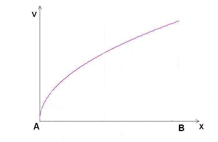
FIGURE \(32.\) Velocity as a function of displacement for non-negligible acceleration.
Therefore, the physically sensible description in mathematical terms, now, for high velocities \(v\), where acceleration \(a\) can be neglected and the curve similar to FIGURE 32 should show a plateau (not shown in FIGURE 32, is provided by \(F_{real} = ma + \frac{mv^2}{2 x}\), eq.(\ref{FIRSTOCCURRENCEOFrealforce}), but reordered in its energy form \begin{equation} \label{realforceathighv} F_{real} x = ma x + \frac{mc^2}{2}, \end{equation} which, having in mind that \(ma x = \frac{mc^2}{2}\) due to eq.(\ref{forcecomponentequality}), becomes \begin{equation} F_{real} x = mc^2, \end{equation} which is \begin{equation} \label{energyequation} \boxed{E = mc^2}, \end{equation} where \(E\) is the energy of a body of mass \(m\) which moves at a limiting velocity \(c\).
Thus, there is another quantity at high \(v\), characterizing the motion of the bodytwice the kinetic energy. Consequently, at high \(v\) force loses its meaning as a quantity characterizing motion (Newton, Maxwell, Lorentz) and motion of the free body is already characterized by energy Leibnitz. At high velocities, the motion is described by a different equation; namely, eq.(\ref{energyequation}), not by eq.(\ref{FIRSTOCCURRENCEOFrealforce}).
Also, because at high velocities there is no acceleration, the character of motion turns into uniform translatory motion, which is akin to rest. Notice that, at high velocities, while uniform translatory motion has preserved the spatial displacement, it is deprived of the second characteristic of real, operative, motionthe inevitable velocity change when a free body is acted upon by a constant force. Thus, we started from rest, then went through motion and ended again at a state akin to rest.
The above shows that the mass-energy relation \(E = mc^2\), which the absurd relativity cannot derive in principle (cf. also here and here), despite the massive propaganda that it does, is inherent in classical physics. The classical origin of \(E = mc^2\) was already shown here, where it was demonstrated that \(E = mc^2\) exists in classical electrodynamics as the expression of Amperes law.
Although this was discussed earlier, a remark may be due here as well, showing that physics cannot emerge from purely formal considerations. Thus, here is another example where mathematics cannot substitute physical considerations. Of course, because of \(v^2 = 2ax\), we can write, instead of \(Fx = max + \frac{mv^2}{2}\) the equality \begin{equation} Fx = m\frac{v^2}{2} + \frac{mv^2}{2}, \end{equation} which is \(Fx = mv^2\), or \(E = mv^2\), and one may remain with the impression that the concept of force disappears even at medium velocities, where motion can be expressed only via energy, and the notion of force loses meaning even at medium velocities. However, from physical considerations, acceleration, \(a\), cannot be neglected at medium velocities, as was already noted. Therefore, for medium velocities we must write the equation for force the way it emerges from \(F = ma\), with acceleration present, but also considering the kinetic energy term, as the correction of DAlembert principle, eq.(\ref{correctedDAlembert}), requires. Neglecting of acceleration may take place only at high velocities, where velocity overwhelms acceleration. It is only at high velocities where we may write \(E = mc^2\).
As
a matter of fact, if one needs to see Newtons second law in its
energy expression, the expanded form of Newtons second law in the
form of \(Fx = mv^2\) provides such opportunity, instead of
relegating to the calculus of variations in the form of variation of
the integral \(\delta \int\limits_{t_0}^{t_1} (T - V) dt = 0\), an
integral which we will be the topic of short discussion here.
Considerations regarding mass-energy relationship \(E = mc^2\)
According to \(E = mc^2\), eq.(\ref{energyequation}), the energy of a body of mass \(m\) at very high velocities only depends on its masseach mass \(m\) has its corresponding maximum energy which cannot be surpassed.
The physical content of \(E = mc^2\), eq.(\ref{energyequation}), excludes having energy without matter on one hand, and on the other, it excludes the equivalence of energy and matter in the sense that energy can be converted into matter and vice versa. Eq.(\ref{energyequation}) can only serve as a formal measure of energy in terms of mass multiplied by the square of the speed of light.
Eq.(\ref{energyequation}) has nothing to do with what is passed as interpretation, offered by the senseless so-called relativistic physics, whose absurdity was already proven unequivocally here. The equation \(E = mc^2\) only shows that at high velocities, Newtons second law loses meaning. Furthermore, the notion of infinite mass also loses meaning altogether in the presented correct physical content of \(E = mc^2\), eq.(\ref{energyequation}).
We would emphasize in the present context once again, that force, expressed as \(F = ma\), characterizes motion only at velocities close to zerothe usually considered Newtons second law; that is, the limited form of Newtons second law, is only valid for velocities practically equal to zero. Further, because at high velocities acceleration is negligibly small, Newtons second law is inapplicable. At high velocities force loses its meaning, and motion is already characterized solely by energy. Of course, at medium velocities motion is characterized by both force and energy.
It should also be noted that the constant velocity \(c\), which velocity \(v\) turns into at high \(x\), is not velocity of light in the general case. The constant \(c\) will be speed of light only when it pertains to electromagnetic waves (cf. Amperes law as an expression of \(E = mc^2\) here). In all other cases, constant velocity \(c\) will have a specific value, corresponding to the free body studied.
Action in Classical Physics
Action and Uncertainty RelationsFundamental Notions and Properties of Classical Physics
Despite the impression created, that action (other than the least action principle) and uncertainty principle\(^{87}\), are arrived at only in quantum mechanics, in contrast to the claimed lack of uncertainty relations in classical mechanics, we will show that, in fact, action, and the uncertainty principle connected with it, are primarily inherent attributes of classical mechanics, and their presence in quantum mechanics, if one should pay attention at all to a discipline already shown to be non-scientific, is no more than a rudimentary signature of quantum mechanics as misunderstood classical mechanics.
Expectedly, we will observe the arrival at the concept of action in classical physics only when there is operative motion; that is, only when there is acceleration.
Therefore, we cannot expect the concept of action to follow from the analysis of the usual, limited form of Newtons second law, eq.(\ref{Newtonssecondlaw}), because it is an equation of restcf. here. Limited classical action is impossible because, when \(F = ma\) there is no real displacement \(\Delta x\). One, however, is tempted to multiply both sides of \(F = ma\) by \(\Delta t \Delta x\) purely formally. However, because \(\Delta x = 0\), we end up with \(0 = 0\). In conclusion, as said, action can only be observed with \(F_{real}\).
Presence of action may be expected only in the expanded form of Newtons second law, eq.(\ref{FIRSTOCCURRENCEOFrealforce}), on the one hand, and on the other, classical action is arrived at from the most fundamental equation of classical mechanics; namely, \(v^2 = 2ax\), eq.(\ref{basiclawofmechanics}), which pertains to motion of a free body impelled by a constant force. It should be recalled, however, that the expanded form of Newtons second law \(F_{real} = ma + \frac{mv^2}{2 x}\), eq.(\ref{FIRSTOCCURRENCEOFrealforce}), is derived here, in an absolute way, from the most fundamental law of mechanics \(v^2 = 2ax\), eq.(\ref{basiclawofmechanics}). Therefore, although we will first discuss the notion of action in what follows from \(F_{real} = ma + \frac{mv^2}{2 x}\) as it was derived from the critique of DAlemberts principle, nonchalant about the absoluteness of the expression for \(F_{real}\), the definitive discussion, the discussion based on the absolute equality \(v^2 = 2ax\), begins here.
The quantity known as action is said to play a prominent role in quantum mechanics, and is even considered as its epitome. It is thought to be symbolized by the Planck constant \(h\). Mere presence of the elementary quantum of action \(h\) in a formula, is considered the divide, indicating that we are already dealing with quantum physics. It was seen on page, however, that the introduction of \(h\) miserably failed from the very first attempts at introducing quantum mechanics.
On the other hand, it was seen from C. I. Noninskis classical derivation of the blackbody radiation formula\(^{11}\), presented here, that the correct physical picture of the mechanism of blackbody radiation is gathered around the average exchanging energy (heat) which the parts of the system transfer among themselves. This leads naturally to a constant, \(\mathscr{h} \, \, \), however of correct physical origin, compared to the physically confused origin of Plancks \(h\), notwithstanding the fact that the value of the correctly understood origin of said constant is calculated from the experimental data in the same way as is done in \(\S11\) and \(\S12\) of paper\(^{11}\).
Interestingly,
however, as will be seen, when correctly analyzing motion in classical
mechanics, especially when honoring the principle of inevitable
non-zero velocity change during real displacement of a free body
acted upon by a constant force, stemming from \(v^2 = 2ax\), it
is further revealed that not only is actionper se, \(W\), but
the elementary quantum of action itself, \(\Delta w\), also an
inherent feature of classical mechanics. The exact meaning of \(W\)
and \(\Delta w\) will become clear shortly.
Classical Action
Despite the fact that the equation for the real force \(F_{real} = ma + \frac{mv^2}{2 x}\), eq.(\ref{FIRSTOCCURRENCEOFrealforce}), follows directly from the absolute equality \(v^2 = 2ax\), eq.(\ref{basiclawofmechanics}), as seen here, and therefore we may discuss action only stemming from that absolute equality \(v^2 = 2ax\), as is done here, we will begin the analysis with the expanded Newtons second law, which was arrived at from the correction of DAlembert's law, eq.(\ref{correctedDAlembert}) \begin{equation*} A = (F_{real} - ma) \Delta x = \frac {mv^2} {2}, \end{equation*} not even suspecting that the expanded Newton law has an absolute, indisputable character (in this form of writing, for clarity here, we change the notation of the interval \(x\), writing it as \(\Delta x\)) \begin{equation}\label{energyexpressionwithdelta} A = \left(F_{real} - m\frac{\Delta v}{\Delta t}\right) \Delta x = \frac {mv^2} {2}. \end{equation} It is obvious that the lucky circumstance that the acceleration \(a\) is constant, as was accepted in this analysis, allows us to express it as \( a = \frac{\Delta v}{\Delta t} \), instead of as \(a = \frac{dv}{dt}\). From eq.(\ref{energyexpressionwithdelta}) we get: \begin{equation*} F_{real} \Delta x = m \frac{\Delta v}{\Delta t} \Delta x + \frac {mv^2} {2} \end{equation*} \begin{equation} \label{actionfromcorrectedNewton} F_{real} \Delta x{\Delta t} = m \Delta v \Delta x + \frac {mv^2} {2} \Delta t \ \ [ J \ s ], \end{equation} obtaining an equation containing the combined effect of the force both in time and in space. What is obtained is a classical expression of action, in its only possible form when it comes to the studied case of a free body induced into motion by a constant force, stemming from the expanded force formula \(F_{real} = ma + \frac {mv^2} {2 \Delta x}\).
Thus, instead of Newtons second law, which is said to characterize motion by the quantity called impulse (\(F \Delta t\)) (equal to change of momentum), the law which expresses the real motion, is characterized by the quantity called action (\(F_{real} \Delta t \Delta x\))\rm \normalfont, which includes both change of momentum and change of energy.
Notably, action in classical physics, a quantity characterizing motion, explored at medium velocities, can only appear as a combination of momentum-position and energy-time expression.
Therefore, again, instead of Newtons law, which is said to characterize motion by the quantity called impulse (\(F \Delta t\)) (equal to change of momentum), the law which expresses the real motion is characterized by the quantity called action (\(F_{real} \Delta t \Delta x\)), which includes both momentum and energy.
Furthermore, eq.(\ref{actionfromcorrectedNewton}) can also have an alternative meaning. Indeed, notice that the above expression of action, stemming from \(F_{real}\), while preserving the same form, now can be seen as expressing both momentum-position and energy-time uncertainty relations: \begin{equation*} \label{} F_{real} \Delta t \Delta x = m \Delta v \Delta x + \frac {mv^2} {2} \Delta t \ = \end{equation*} \begin{equation} \label{classicalactionfromrealforce} \Delta p\Delta x + \Delta E \Delta t \ne 0 \ [J \ s]. \end{equation} It is to be noted that, in fact, in practice, when eq.(\ref{actionfromcorrectedNewton}) is treated as an expression of classical action, both terms on the right side of eq.(\ref{classicalactionfromrealforce}) determine action, but we always separate these terms for convenience (REMARK: while the dimensions \([J\ s]\) are obvious for \(\Delta E \Delta t\), please see footnote\(^{88}\) that the dimensions of \(\Delta p \Delta x\) are also \([J\ s]\)).
In other words, as a reminder, we always observe the effect of force either in time, and that effect (the impulse) had been thought by some to be the measure of motion (Galileo, Newton, Lorentz), \begin{equation} \label{} F \Delta t = m \Delta v, \end{equation} or only in space (during a displacement) and others (Leibnitz) had thought that energy \begin{equation} \label{} F \Delta x = \frac {mv^2} {2}, \end{equation} which follows, is the measure of motion.
As said, especially in solving engineering problems, we practically never take into consideration that the real effect of force (which besides considering motion as mere spatial displacement, also includes qualitative transformation; namely, change of velocity) takes place simultaneously both in time and in space, as in \(\Delta p \Delta x + \Delta E \Delta t \ne 0\), eq.(\ref{classicalactionfromrealforce}).
Also, because of \(ma = \frac {mv^2} {2 x}\), eq.(\ref{forcecomponentequality}), we have (considering \(\Delta\)'s) \begin{equation*} m \frac{\Delta v}{\Delta t} = \frac{m \Delta v^2}{2 \Delta x} \end{equation*} \begin{equation*} m \Delta v \Delta x = \frac{m \Delta v^2}{2} \Delta t \end{equation*} \begin{equation} \boxed{\Delta p \Delta x = \Delta E \Delta t}. \end{equation} Thus, interestingly, not only is the real force a combination of momentum-position and energy-time effect, but these two effects are equal to each other.
Further, in this part of the discussion we will again use the equality \(ma = \frac {mv^2} {2 x}\), eq.(\ref{forcecomponentequality}), which, as seen, allows us to write \(F_{real} = ma + \frac{mv^2}{2 x}\), eq.(\ref{FIRSTOCCURRENCEOFrealforce}), also as \begin{equation*} F_{real} = \frac{mv^2}{2x} + \frac{mv^2}{2x} = \frac{mv^2}{x}, \end{equation*} \begin{equation}\label{Frealmv2overx} \boxed{F_{real} = \frac{mv^2}{x}}. \end{equation} As we saw, eq.(\ref{Frealmv2overx}), reordered, brought about, here, a most astounding result.
In this discussion here, however, we will not deal with the really important astounding result, seen here, but will satisfy ourselves by using \(F_{real} = \frac{mv^2}{x}\), eq.(\ref{Frealmv2overx}), to only observe that, by multiplying both sides by mass \(m\), and reordering, from that equation the momentum \(mv\) as a function of \(x\) becomes \begin{equation}\label{momentumasafunction of x} mv = \sqrt{F_{real}mx}. \end{equation} It was already discussed, seen there as eq.(\ref{trial momentum}), in proving the absolute character of the expression of \(F_{real}\), that eq.(\ref{momentumasafunction of x}), which arrives from the expanded Newton second law, is not only a perfectly legitimate offspring of that expanded law, but is also an absolute equality. Here, we will pretend that we are unaware of the absoluteness of that law and will use eq.(\ref{momentumasafunction of x}) for the purposes of analyzing its graphical representation, as if that equation has only arrived from the expanded Newton second law, stemming from the corrected DAlembert principle. Later, we will analyze the graphical representation of momentum, plotted against displacement, coming straight from the absolute equality \(v^2 = 2ax\), with no evident connection with any discovered law in physics, such as Newtons second law of motion. The use of \(v^2 = 2ax\) guarantees unequivocally that what is being analyzed is motion in its true, operative sense. Of course, expectedly, the conclusions which we will draw later from the graphs based on the absolute equality \(v^2 = 2ax\), will be the same as the conclusions we will now draw from the \(mv = \sqrt{F_{real}mx}\) variant of the expanded Newton second law, without realizing its absoluteness, only perceiving it as a correction of an already discovered law.
Graphs of \(mv = \sqrt{F_{real}mx}\) simplified as \(mv = \sqrt{mx}\) for \(F_{real} = 1\) analyzed
FIGURE
33 shows the one-dimensional motion along the x-axis, described by
\(p_x = mv_x\) from eq.(\ref{momentumasafunction of x}), plotted
against \(x\), for \(F_{real}=1N\) and two different values of \(m\).
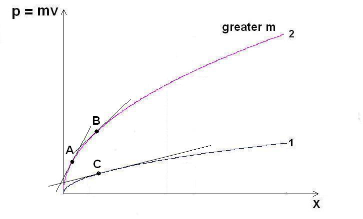
FIGURE \(33.\) Family of trajectories, expressing the absolute relation \(mv = \sqrt{mx}\), for accelerating bodies at constant acceleration as a result of application of \(F_{real} = 1N\) force, of two values of \(m\) (curves 1 and 2) (Note: constant \(a\) but different \(m\) means that the forces acting, resulting in trajectories 1 and 2, are different).
It is seen from FIGURE 33 that the slope \(\frac{dp}{dx}\) at every point of each well-behaved curve in Fig.33 is non-zero\(^{89}\). For \(m = 1\), and already accepted \(F_{real} = 1\) unit of force, the derivative of eq.(\ref{momentumasafunction of x}) is \(\frac{dp}{dx} = \left( \sqrt{x} \right)' = \left( x^{ \frac{1}{2}} \right)' = \frac{1}{2} x^{ \left( \frac{1}{2} - 1 \right)} = \frac{1}{2} x^{ - \frac{1}{2}} = \frac{1}{2 \sqrt{x}} > 0\). However, the fact that the derivative \(\frac{dp}{dx}\) is not zero also means that both \(dp\) and \(dx\) are themselves non-zero as well, which further means that their product is also non-zero \begin{equation} \label{differentialofclassicalaction} dxdp = dw \ne 0. \end{equation} The fact that the product \(dp dx\), eq.(\ref{differentialofclassicalaction}), is not zero, has an important physical meaning. It means that, along the classical trajectory of the classically moving body, there will inevitably be a non-zero quantity in classical mechanics, characterizing the motion of the body, which has been thought, for over a century, to be an attribute only of quantum mechanics (as far as the principle of least action in classical mechanics goes, it will be discussed subsequently). The product \(dxdp\) has the dimensions of the important quantity characterizing motion, called action. Thus, eq.(\ref{differentialofclassicalaction}) comprises the elementary quantum of action in classical mechanics. The above are inherent properties of the very fundament of classical mechanics.
It may be clearer, more intuitive and instructive, to alternatively observe the small intervals along the trajectory of bodys motion as \(\Delta x\), as well as \(\Delta p\), instead of the usual writing of these intervals as \(dx\) and \(dp\), also realizing that \(\frac{dp}{dt}\) is, in fact, the limit \begin{equation} \frac{dp}{dt} = \lim_{\Delta t \rightarrow 0} \frac{\Delta p}{\Delta t} \end{equation} of the quotient of these two quantities, whose denominator tends towards zero in the limit. These are real intervals, which are necessarily non-zero, when the observed free body moves.
Consequently, when the free body moves under the action of a constant force, the product of \(\Delta x\) and \(\Delta p\), must also necessarily be non-zero; that is, \begin{equation}\label{classicalactiondeltaw} m\Delta v \Delta x = \Delta p \Delta x = \Delta w \ne 0, \end{equation} the same way the product of the differentials \(dp dx\) in eq.(\ref{differentialofclassicalaction}) is non-zero.
As mentioned in another section below (here and on), eq.(\ref{classicalactiondeltaw}) will also be observed as an expression for the uncertainty relation, which that same classical physics has failed to consider thus farthe presence of uncertainty relations (momentum-position and energy-time) is being relegated by the mainstream only to the misunderstood classical physics, called quantum mechanics.
In eq.(\ref{classicalactiondeltaw}), \(\Delta p\) is the change of momentum (the impulse) during the real displacement of the particle from point \(a\) to point \(B\) in space, while \(\Delta x\) is the change of the x-axis coordinate during the displacement. The quantity \(\Delta w\) is the action, corresponding to the change of momentum coordinate during the displacement from spatial point \(a\) to spatial point \(B\)cf. FIGURE 34.
Similarly to eq.(\ref{differentialofclassicalaction}), the minimal value of quantity \(\Delta w\), eq.(\ref{classicalactiondeltaw}), is the elementary quantum of action, derived purely classically\(^{90}\).
Now, as was already emphasized, if we really have to consider motion of a free body and not the body at rest, then we must observe a finite interval of displacement, not just one point of the x-axis.
What FIGURE 33 shows can be understood by recalling that \(x\) signifies \(\Delta x\), whereby the initial value of \(x\) is zero. Therefore, FIGURE 33 depicts the change of momentum as the length of the interval \(\Delta x\) increases. Thus, FIGURE 33 cannot be used, as it may appear at first sight, to demonstrate that for an exact \(x\) the value of \(p\) can be determined exactlyFIGURE 33 has nothing to do with the determination (measurement) of \(x\) and \(p\); it only shows what \(x\) and \(p\) of a free body really are when that free body is acted upon by a constant force. Notice, however, that the various positions and momenta along \(\Delta x\) can be measured with various uncertainties which we denote in the same way, as \(\Delta x\) and \(\Delta p\). The confusion in the notation can be avoided by following the context. We avoid using \(\Delta x\) to denote the interval of \(x\) because it may cause a greater confusion, mixing it up with virtual displacement, while here we are only observing real displacement. The intervals \(\Delta x\) (or \(x\), as we denote it), as well as \(\Delta p\) (or \(mv\), as we denote it), are real intervals, which are necessarily non-zero, when the observed free body moves.
Further,
as can be seen in FIGURE
34, where the two curves, stemming from the reordered variant
\(mv = \sqrt{F_{real}mx}\), eq.(\ref{momentumasafunction of x}), of
the expanded Newtons second law \(F_{real} = ma + \frac{mv^2}{2 x}\),
eq.(\ref{FIRSTOCCURRENCEOFrealforce}), are plotted for two different
values of \(m\), ceteris paribus, the elementary quantum of
action \(\Delta w = \Delta x \Delta p\) becomes all the more
negligible with the increase of \(m\) at a given \(\Delta p\) or for
the same interval \(\Delta v\) with the increase of coordinate \(p\)
for a given \(m\)at a given \(\Delta p\) the value of \(\Delta x\) is
greater for the lower value of \(m\).
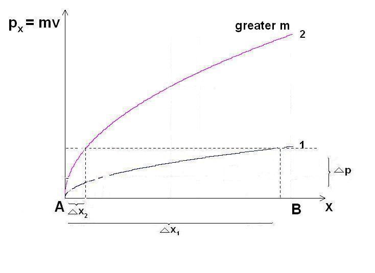
FIGURE \(34.\) Same as FIGURE 33 but with broken lines drawn to indicate what \(\Delta x\) would be at a constant \(\Delta p = \Delta (mv)\)}.
It is seen from FIGURE 34, which arrives from expanded Newtons law in the form \(mv = \sqrt{F_{real}mx}\), not from the absolute equality \(v^2 = 2ax\), which will be analyzed separately below, that the indeterminacy of position begins to be more expressed in the micro-world, just as quantum mechanics attempts to claim (attempts, because the claim of a non-physical doctrine such as quantum mechanics is nothing other than inconsistency, and therefore should make itself scarce in any scientific discourse); however, this fact is now observed in classical mechanics, without any aid from quantum mechanics.
Conversely, for a given \(m\) and a given \(\Delta p\), the elementary quantum of action, \(\Delta w\), increases with the increase of \(v\).
In other words, for a given \(\Delta p\) around a given \(p\), the coordinate \(x\) is determined with a greater accuracy at a higher \(m\); the uncertainty along \(x\) decreases with the increase of \(m\) and practically disappears at high \(m\); graininess (read some more on graininess in the footnote\(^{91}\)) disappears at high \(m\). The opposite is observed at lower \(m\), lower \(v\) and weaker force, where the graininess begins to show itself. This conclusion; namely, that quantum effects, their graininess, show themselves the more the micro-world comes to the fore and vice versa, is standardly ascribed to quantum mechanics, but, as can be seen from FIGURE 34, this phenomenon is indelibly present, this phenomenon is inherent, in classical mechanics when the expression of force is \(F_{real} = ma + \frac{mv^2}{2x}\), as corrected in the course of the derivation of eq.(\ref{FIRSTOCCURRENCEOFrealforce}), providing the hitherto unappreciated full description of force, considering true motion in its operative sense.
Also, for a given \(m\) and \(\Delta p\), the inaccuracy of determining the position \(x\) increases with the velocity. In other words, the more removed from rest a body is, the less accurately its position can be determined while keeping the same momentum change.
Action in its purest formaction from \(v = \sqrt{x}\)
So far, classical action was derived from the expanded Newton second law, as it was derived from correcting the DAlemberts principle, oblivious to the fact that said expanded law is an absolute relationship. These derivations led to revealing very valuable, hitherto unrecognized sides of classical mechanics characterizing motion. Especially valuable was the finding here, that the expanded Newton second law leads to the combined momentum-position and energy-time uncertainty relations \(\Delta p_x \Delta x + \Delta E \Delta t \ne 0\).
In
this part of the book, we will go beyond even the expanded Newton
second law and will consider the absolute generator of that lawthe
absolute equality \(v^2 = 2ax\) (cf. here),
which is the result of absolute truths in physics, as seen here.
Apropos, it must be prominently emphasized, following from the proof here,
that it is the expanded Newton second law \(F_{real} = ma +
\frac{mv^2}{2 x}\), eq.(\ref{FIRSTOCCURRENCEOFrealforce}), that is
derived from the absolute equality \(v^2 = 2ax\) defining motion, not
its limited form \(F = ma\), which is actually a law of rest, as seen
here. Therefore, the fact
that not the limited Newtons law \(F = ma\), but the expanded
Newtons law is the law \(F_{real} = ma + \frac{mv^2}{2 x}\) is the
law that arrives from absolute principles, makes the latter law
unquestionable as the law expressing the full meaning of force.
Proving that the absolutely true equality \(v^2 = 2ax\) is, actually, an expression of \(F_{real} = ma + \frac{mv^2}{2 x}\)an interesting exercise
That \(F_{real} = ma + \frac{mv^2}{2 x}\) stems from the absolute equality \(v^2 = 2ax\) was already definitively proved here. However, we will, as an exercise, prove that stemming from a slightly different perspective.
Thus, start with what was derived here, based on the absolutely true definitions of velocity and acceleration \begin{equation*} v^2 = 2ax, \end{equation*} multiply both sides by \(m\) \begin{equation*} mv^2 = 2max, \end{equation*} and reorder it as \begin{equation*} 2ma = \frac{mv^2}{x} \end{equation*} \begin{equation}\label{resemblesNewton} 2ma = \frac{mv^2}{2x} + \frac{mv^2}{2x}. \end{equation} Eq.(\ref{resemblesNewton}) is an absolutely true equality which cannot be questioned for any reason.
On the other hand, any equalities that may possibly be claimed, involving the same quantities, which may be reduced to eq.(\ref{resemblesNewton}), are guaranteed to be absolutely true equalities. Moreover, any equality containing the quantities participating in eq.(\ref{resemblesNewton}), must, in the end, display the same functional relation as the functional relation expressed by eq.(\ref{resemblesNewton}) when it comes to a free body acted upon by a constant force. Therefore, even if we didn't know the expression \(F_{real} = ma + \frac{mv^2}{2 x}\) for the real force, in order to rely on that expression for guidance, we can immediately see that the dimensions on the left side of the equality in eq.(\ref{resemblesNewton}) are \(\left[ \frac{kg \ m}{s^2} \right] = \left[ N \right]\), which means force. Despite the name Newton given to the unit \(\left[ N \right]\), one may not have even heard about the history of that unit. Suffice it to know that \(\left[ N \right]\) is a unit of force.
Obviously, \(\frac{mv^2}{2 x}\) must also be expressed in \(\left[ N \right]\), which it really is \(\rightarrow\left[ \frac{kg \ \frac{m^2}{s^2}}{m} \right] = \left[ \frac{kg \ m}{s^2} \right] = \left[ N \right]\).
Now, if \(\frac{mv^2}{2 x}\) is force, which it really is, and if the double of it is \(2ma = \frac{mv^2}{x}\), as eq.(\ref{resemblesNewton}) indicates, then half of it, \(\frac{mv^2}{2 x}\) is equal to \(ma\), which we may substitute in eq.(\ref{resemblesNewton}), to obtain \begin{equation}\label{derivedexpandedNewton} \mathscr{F} = ma + \frac{mv^2}{2x}. \end{equation} Notice, eq.(\ref{derivedexpandedNewton}) is reached only based on the analysis of the absolute equality, eq.(\ref{resemblesNewton}), describing motion. It is only based on definitions of physics, which, as being definitions, are absolute truths of physics. Eq.(\ref{derivedexpandedNewton}) has nothing to do with additional discoveries in physics such as, for example, Newtons second law, limited or expanded.
When looking at eq.(\ref{derivedexpandedNewton}), however, it is at once obvious that \(\mathscr{F} = ma + \frac{mv^2}{2x}\) is exactly the same relationship as \(F_{real} = ma + \frac{mv^2}{2 x}\), eq.(\ref{FIRSTOCCURRENCEOFrealforce}), the former derived on absolute premises, while the latter derived in a completely different way here, based on achievements of physics, which can in principle, be under scrutiny, no matter how well established they may be considered. Therefore, \(\mathscr{F} = F_{real}\), Q.E.D.
Consequently, aside from even mentioning relativity, unequivocally exposed as absurdity, with no place in physics (cf. as well), we should not only not say that someone is working in the realm of Newtonian mechanics, but from now on, we should only talk about fundamental laws of mechanics, which are absolute, and work within these laws, rather than even mentioning the term Newtonian mechanics in any context of classical physics. In this book, however, we will keep using the name expanded Newtons second law for the relationship \(F_{real} = ma + \frac{mv^2}{2 x}\) out of respect for the great scientist, while, the real truth is that, as was seen, that relationship stems from inherent absolute truths of physics.
Here, unlike what we did earlier, basing the discussion on the limited and expanded Newton second law, we will observe the measure of motion, which is the classical action, and the related classical uncertainty relations, as they arrive in the purest, most unquestionable possible way; namely, from absolute truths of physics.
The analysis of action, based on the absolutely true relation \(v^2 = 2ax\), shows the same characteristics, which we saw displayed by the expanded Newton second law. Such coincidence is most natural and expected, because the expanded Newton second law is an outgrowth of that absolute relationship. Therefore, some of the conclusions may seem annoyingly repetitive. However, it must not be forgotten, that the effects following from \(v^2 = 2ax\) are primary. They exist prior to the discovery of any further laws such as, for example, the so-called Newtons laws of motion (which were seen to actually be laws of restcf. here.
Classical action and classical uncertainty principle can be seen directly from the graphical illustration of the above-discussed free body and the fundamental law \(v^2 = 2ax\) of its motion under the impact of a constant force, an absolute equality derived here. It is nothing but incredible what conclusions can be reached when one observes carefully only the very definitions of velocity and acceleration. It is hard to believe that such significant effects, described in this book, emerging from absolute truths of physics, have remained hitherto undetected, especially because these phenomena are attributes of the very fundamental definitions of physics, not requiring any additional discoveries and knowledge.
Some of the effects seen in FIGURE 34 are briefly mentioned below, while immediately after that, here, a numerical example will commence, based on the absolute equality \(v^2 = 2ax\). The numerical example gives an even clearer picture of the universality of the phenomena discussed, a universality hardwired into even the formal structure of physics. We may note that here we are experiencing a lucky circumstance when a mathematical expression fully serves physics, which is not at all the case for the totality of the mathematical equations. Also, practically all the effects observed in the expanded Newton second law; that is, all the effects based on the laws of physics concerning motion of a free body propelled by a constant force, are discerned in the formally plotted graphs of parabolae. Of course, without the physical meaning, which evolves from these parabolae, the conclusions from a purely formal point of view, make little sense. Nevertheless, the graphs here, are an example as to how useful the formal illustrations can be for understanding concepts.
Here are some observations, based on FIGURE 34. These observations will be made more elaborate and illustrative in the section beginning here, concerning the mentioned parabolae describing motion of a free body, acted upon by a constant force.
Discussion concerning \(2max = mv^2\) in its absolute context
In order to tie up eventual loose ends in this context, that might arise due to the fact that at high velocities, \(v\), acceleration, \(a\), is zero, before going further with discussing the effects seen in the parabolae depicting the absolute equality \(v^2 = 2ax\) (or its shortened form \(v = \sqrt{x}\)), we will comment once again, but in the current context of already being immersed in the absoluteness of this relationship, on the issue brought about earlier, here, during the discussions of the energy expression \(F_{real}x = max + \frac{mv^2}{2 }\) of the expanded Newtons law pertaining to real force \(F_{real} = ma + \frac{mv^2}{2 x}\), eq.(\ref{FIRSTOCCURRENCEOFrealforce}), whose absoluteness was not yet evident at that point.
Thus, when seeing the equality \(2max = mv^2\) one may ask oneself, the same way this question appeared here, when \(F_{real}x = mv^2\) was construed to turn into \(E = mc^2\) at high velocitieshow this happened, when in the same breath it was stated that at high velocities acceleration \(a\) becomes negligible with the increase of velocity \(v\)? Wouldnt the disappearance of \(a\) negate \(2max\), thus rendering the whole equality \(2max = mv^2\) moot?
To answer these question, we must remember that we are discussing physics, not mathematics. Thus, from physical considerations, in order to reach the conclusion that the chain of equalities \(F_{real}x = 2max = mv^2\) turns into \(E = mc^2\) at high velocities, we had to work with the energy expression \(F_{real} x = max + \frac{mv^2}{2}\), stemming from the expanded Newton second law \(F_{real} = ma + \frac{mv^2}{2 x}\), eq.(\ref{FIRSTOCCURRENCEOFrealforce}), because if we worked directly with \(F_{real} = ma + \frac{mv^2}{2 x}\), the expression for real force \(F_{real}\) would lose meaning at high velocities where \(a\) becomes negligible.
On the other hand, however, when, instead of the expression for the real force \(F_{real}\), we use the energy expression \(F_{real}x\), we see that in said energy expression \(F_{real} x = max + \frac{mv^2}{2}\) (not in the plain real force expression \(F_{real} = ma + \frac{mv^2}{2 x}\), in which the neglect of \(a\) at high velocities causes both terms on the right of the equality to vanishthese two terms; namely \(ma\) and \(\frac{mv^2}{2 x}\), being on top of it, equal to each other, as shown here its left side represents energy even at medium velocities. Again, the left side of \(F_{real} x = max + \frac{mv^2}{2}\), which, because of \(ma = \frac {mv^2} {2 x}\) seen here, is \(F_{real} x = mv^2\), comprises energy.
Furthermoreto
add resolution to the problem concerning finiteness of both sides of
\(F_{real} x = mv^2\)quite significantly, the right side of
\(F_{real} x = mv^2\) cannot be neglected, even more so at high
velocities. Therefore, we know that the right side of \(F_{real} x =
mv^2\) not only cannot be neglected, but it must be energy \(E\).
Hence, for extreme velocities we got \(E = mc^2\). So, no matter how
uncertain we are (we shouldnt be) about the left side of \(F_{real} x
= 2max = mv^2\), because of \(F_{real}\) containing \(a\); that is,
containing constant acceleration \(a\), which at high velocities must
be neglected (but, as said before, \(x\) is large), we know already
that the right side, \(mv^2\) must have the meaning of energy. Also,
we know that at high velocities, when \(a \approx 0\), \(v\) becomes
\(c = const\). We substitute that \(c\) in \(E = mv^2\), and get
finally \(E = mc^2\).
Effects seen in FIGURE 35
FIGURE
35 looks just like FIGURE
34. However, FIGURE
34 is based on the expanded Newton law, when its absoluteness
was not suspected, while FIGURE
35 depicts graphically the absolute equality \(v^2 = 2ax\),
reshuffled as \(mv = \sqrt{2m^2ax} = \sqrt{F_{real}mx}\), plotted for
\(F_{real} = 1\) unit of force, which is \(mv = \sqrt{mx}\).
FIGURE \(35.\) Same as FIGURE 33 and FIGURE34, but broken lines drawn to indicate what \(\Delta x\) would be at a constant \(\Delta p = \Delta (mv)\)
Here we will give an initial idea about these effects, which will be elaborated on in the next section of this book (here), and, of course, the effects which will be established will be the same as the effects we determined when we pretended we dont know that the expanded Newton second law \(F_{real} = ma + \frac{mv^2}{2 x}\), eq.(\ref{FIRSTOCCURRENCEOFrealforce}), is an absolute relationship.
Effects at a Given \(\Delta p\) and a Given \(m\)As any parabola, the parabola \(v = \sqrt{x}\) (whereby, in the latter formula, also \(m = 1\)) shows that at a given \(\Delta v\) the corresponding \(\Delta x\) increases with velocity \(v\). This parabola, describing a real physical trajectory, implies a physical meaning. Thus, for a given \(\Delta v\), the inaccuracy of determining the position \(x\) increases with the velocity \(v\). In other words, the more removed from rest is a body, the less accurately can its position be determined.
This further leads to the observation that, obviously, because of the increasing \(\Delta x\) with \(v\) at a given \(\Delta p\), the elementary quantum of action, \(\Delta w\), increases with the increase of \(v\).
We already observed these effects when discussing the expanded Newton law and we are reconfirming them here for the case of the absolute equality of mechanics.
Effects at a Given \(\Delta p\) and Varying \(m\)The value of \(\Delta x\) is greater for the lower value of mass \(m\). Indeterminacy of position begins to be more expressed in the micro-world, just as quantum mechanics claims. However, this fact is now observed in classical mechanics, not only without any aid from quantum mechanics but also follows from an absolute equalitythe absolute equality \(v^2 = 2ax\) emerging from absolute definitions of physics; namely, the definitions of velocity and acceleration. In other words, for the same \(\Delta p\), at a greater \(m\), the x-axis coordinate is determined with a greater accuracy (for the same \(\Delta p\), the uncertainty along the x-axis decreases with the increase of \(m\) and practically disappears; graininess disappears). The opposite is observed at lower \(m\), where the graininess begins to show itself. This conclusion; namely, that quantum effects, graininess, show themselves the more the micro-world comes to the fore and vice versa, is standardly ascribed to quantum mechanics but, as we see, this phenomenon is indelibly present in classical mechanics.
As can be seen in FIGURE 35, the elementary quantum of action, \(\Delta w\), becomes all the more negligible with the increase of \(m\).
GraininessThere was a footnote on graininess above, but we will repeat some of it in this context. From all said so far, it is clear that classical physics has quantum character as its internal characteristic, with its peculiar expressions. For example, it is seen that eq.(\ref{classicalactiondeltaw}); namely, \(m \Delta v \Delta x = \Delta p \Delta x = \Delta w \ne 0\), allows for practically any level of quantization (arbitrary graininess).
We will further explore the quotient \(\frac{\Delta w}{W}\) and observe how it varies with \(m\), as well as, how \(\frac{\Delta w}{W}\) varies with \(x\), when keeping the corresponding other parameters constant.
It may also be noticed, that in these sections we often do not separate in the discussion action from uncertainty. That is not wrong, because these notions have common elements. However, later in this book there is a section which discusses uncertainty principle on its own.
Firstly, however, we will make the above conclusions more demonstrative.
Numerical Example
Further Analysis of the Graph \(v = \sqrt{x}\) Following from Absolute Truths
Although I am, in principle, not in favor of concrete illustrations with numerical examples of concepts in physics, preferring that the comprehension of these concepts takes place in more abstract terms, in this instance, numerical examples may help in the ruminations on the discussed matter.
To understand how the properties of the parabola have physical meaning, we must first clearly realize that contemporary physics ignores the fact that constant force applied to a free body inevitably causes change of its velocity, hence, causes change of its momentum. In other words, contemporary physics ignores the relationship \(p = m v = m\sqrt{x}\) for a motion of a free body under the action of a constant force.
Notice again, the novelty here, overlooked in contemporary physics, is that force \(F_{real}\) has, in addition to the effect in time, \(ma\), an effect space, \(\frac{mv^2}{2x}\). Recall the conclusion here that spatial effect of force; that is, the new term in \(F_{real}\), is the change of energy per unit of displacement, \(\frac{mv^2}{2x}\), expressed here as \(\frac{ \frac{m\Delta v^2}{2}}{\Delta x}\), while the temporal effect of force is the change of momentum per unit time, \(ma\), the way force \(F\) is originally known, expressed here as \(\frac{m \Delta v}{\Delta t}\).
However, once we heed the absolute equality \(p = m\sqrt{x}\), which,
despite its inauspiciously looking form, actually includes both the
spatial and the temporal effect of force, because that expression came
from the absolute equality \(v^2 = 2ax\), respectively, from the
applied real force \(F_{real}\), we will draw the following crucial
conclusions:
Analysis of action as a function of \(x\) from the curve in FIGURE 36

FIGURE \(36.\) Family of trajectories \(p = mv = \sqrt{m x}\), for accelerating free bodies at constant acceleration \(a = \frac{1}{2} [\frac{m} {s^{2}}]\), of two values of \(m\) for a varying \(v\) (curves 1 and 2) (Note: constant \(a\) but different \(m\) means that the forces acting, resulting in trajectories 1 and 2 are different).
From FIGURE 36 one clearly sees that the slope of the curve closer to the beginning, say, at point A, is greater than the slope of the curve further away from rest, say, at point B.
Thus, if we take some simple arbitrary numbers, just for illustration, on one hand, for lower \(x\), say, at point A, the slope is \begin{equation} \frac{dp}{dx} = 2, \end{equation} or \begin{equation} \label{dxA} dx = \frac{dp}{2}, \end{equation} then, the action at A is \begin{equation} \label{actionA} dw_{_A} = dp dx = dp \frac{dp}{2} =\frac{(dp)^2}{2}. \end{equation} On the other hand, at higher \(x\), say at point B, the slope of the function is lower; namely, \begin{equation} \frac{dp}{dx} = 1, \end{equation} then, \begin{equation} \label{dxB} dx = dp, \end{equation} and the action at higher \(x\), corresponding to B, is \begin{equation} \label{actionB} dw_{_B} = (dp)^2, \end{equation} showing that the action at point B is greater than the action at point A. Therefore, the first thing that has to be noticed in this short exercise is, that the action changes with \(x\), which goes contrary to the constancy of action, assumed by classical physics, when the system changes its generalized coordinates. We will devote some time to discussing the above-observed variability of action in a separate section.
The increase of action, as the motion progresses, from \(dw_{_A} = \frac{(dp)^2}{2}\), eq.(\ref{actionA}), at point A (lower \(x\) region), to \(dw_{_B} = (dp)^2\), eq.(\ref{actionB}), at point B (higher \(x\) region), may lead to the conclusion that this tendency will continue indefinitely. However, the expression \(m v = \sqrt{m x}\), the shownFIGURE 36 is based on, only illustrates the physical state of the body at intermediate velocities. As the motion progresses under the impact of a constant force, the role of acceleration decreases, becoming less pronounced in value compared to velocity, until fading away. The state of the free body under these new circumstances of disappearing acceleration, cannot be described by the equation \(m v = \sqrt{m x}\) any more, because the body would have reached uniform translatory motion. During uniform translatory motion, the velocity (momentum) versus displacement graph will be a horizontal line parallel to the abscissa, having a slope \(0\) because the run of momentum \(p\) with the displacement \(x\) will already be constant. Therefore, because \(p = const\) \begin{equation} \frac{dp}{dx} = \frac{d \ const}{dx} = 0, \end{equation} whence \begin{equation} dx = \frac{dp}{0}, \end{equation} which is undefined, and we cannot form the expression for the action \(dp dx\).
Interestingly, at the other extreme; that is, when the body is at rest, the expression for the action \(dp dx\) cannot be formed either because for \(x = 0\) \begin{equation} \frac{dp}{dx} = \frac{1}{2 \sqrt{x}} = \frac{1}{0} \end{equation} will also be undetermined.
Thus, what must be emphasized again is that in this physical problem we are not dealing with properties of a mathematical function, but will use mathematics where it makes physical sense. Thus, it makes physical sense to describe the physical phenomenon of the operative motion of a particle by \(mv = m\sqrt{x}\) and \(^{32}\), such as FIGURE 36, for illustrating the motion of a free body impelled by a constant force, only for intermediate velocities. At the two extremes, which are akin to each other; namely, rest and uniform translatory motion, the mathematical expression \(mv = m\sqrt{x}\) does not applyboth at rest and at uniform translatory motion acceleration \(a\) is \(0\) and the body is not in operative motion. The curious thing is that when a free body is acted upon by a constant force, it is being transformed from one state of non-operative motion, rest, through the state of increasing operative motion, into another state of non-operative motion, uniform translatory motion.
Thus, one may observe an interesting paradox when considering action as the measure of motion of a free body under the action of a constant force. Obviously, at rest, action is zero. However, although the free body, set in motion by a constant force, increases its action as the motion progresses, in the areas of high velocity, where acceleration begins to vanish in value compared to velocity, action begins to tend to infinity, again starting to get out of operative motion, which signals the kicking in of uniform translatory motion, which is akin to restat high velocities, motion succumbs to its negation, a state akin to rest.
We
will comment on this phenomenon, caused by the vanishing of
acceleration at higher velocities, in the parts below, observing
action while keeping either \(\Delta x\) or \(\Delta p\) constant.
Analysis of the Curve in FIGURE 36, Plotted for Lower \(m\)
When comparing \(dx\), when expressed by \(dp\), at different values of \(x\), it is seen that \(dx\) is lower for lower \(x\)observe FIGURE 36 and compare \(dx = \frac{dp}{2}\), eq.(\ref{dxA}), at point A (lower \(x\)), and \(dx = dp\), eq.(\ref{dxB}), at point B (higher \(x\)). This indicates that certainty in determining \(x\) is lower at higher \(x\)the slower the body moves, the higher the certainty in determining its position (the lower the \(dx\)). The position of a free body can be determined with absolute certainty only when the body is at rest; that is, when also its impulse (the change of its momentum) is zero. The uncertainty mentioned is a big topic on which we will say no more here, but which will be given attention in the sections to come.
However, if the mass \(m\) is lower (curve 1), then, for the same \(x\) region, the certainty in determining \(x\) decreases (\(dx\) becomes greater), compared to a body of greater \(m\). Also, for the same region of \(x\), the action at lower \(m\) is higher, compared to greater \(m\).
Indeed, take point C in FIGURE 36. Say, the arbitrary slope at that point is \begin{equation} \frac{dp}{dx} = \frac{1}{4}, \end{equation} then, \begin{equation}\label{dxC} dx = 4dp, \end{equation} resulting in \begin{equation} \label{actionC} dw_{_C} = 4(dp)^2. \end{equation} It is seen that the uncertainty in determining position \(x\) grows as the mass \(m\) gets smallercompare \(dx = dp\), eq.(\ref{dxB}), at point B (greater \(m\)), with \(dx = 4dp\), eq.(\ref{dxC}), at point C (lower \(m\)).
Also, the action for the same region of \(x\), is larger at a lower \(m\), compared to the action of a free body of greater \(m\)compare \(dw_{_B} = (dp)^2\), eq.(\ref{actionB}), at point B (greater \(m\)), with \(dw_{_C} = 4(dp)^2\), eq.(\ref{actionC}) at point C (lower \(m\)). Action, being the measure of motion, shows that at lower \(m\), motion fades away (motion turns into its negation, the uniform translatory motion, which is akin to rest) sooner, as the motion progresses.
In the next two sections, we will carry out analysis of the \(mv = \sqrt{m x}\) graph, while keeping either \(\Delta x\) or \(\Delta p\) constant. This will bring additional pictorial clarity to the conclusions drawn so far.
Action and Uncertainty in \(\Delta x\) at Constant \(\Delta p\)
Action
in classical physics can be discussed either for \(\Delta x = const\)
or for \(\Delta p = const\). FIGURE
37 allows discussing of action for \(\Delta p = const\). The
difference \(\Delta p\), expresses the spatial effect of force causing
motion, and this is exactly the effect ignored in contemporary
physics. One notices that now we transformed the quantities we are
going to discuss from differentials \(dp\) and \(dx\) to \(\Delta p\)
and \(\Delta x\), because the formulation of the above-observed
effects in terms of differentials can be more illustrative if they are
shown in terms of differences, as in FIGURE
37.
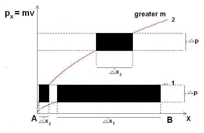
FIGURE \(37.\) The two inevitable curves, stemming from the very definitions of velocity and acceleration, are drawn for two different \(m\), everything else the same. Everything is the same as in FIGURE 33, except that broken lines are drawn to indicate what \(\Delta x\) would be at a constant \(\Delta mv\).
FIGURE 37 illustrates with better clarity the above-discussed absolute phenomena, stemming from the most fundamental equation \(v^2 = 2mx\) of mechanics; namely, that when the spatial effect \(\Delta p\) is kept constant during the motion of a free body under the action of a constant force, the uncertainty \(\Delta x\) in determining position \(x\) grows with the decrease of \(m\) (an effect wrongly claimed to exist only in quantum mechanics) and with the increase of \(x\). With the decrease of \(m\) or increase of \(x\), it takes a longer displacement, in order to achieve a given constant \(\Delta p\). This observation applies for medium velocities. When the motion reaches states, whereby velocity dwarfs acceleration, making acceleration negligible, the constant \(\Delta p = const\) to be explored becomes increasingly narrower, while the observed \(\Delta x\) becomes increasingly wider, until \(\Delta p\) reaches \(0\), while \(\Delta x\) becomes infinite. Of course, for a given finite accuracy the value of \(\Delta p \Delta x\) will approximate zero and action will lose meaning, before getting into mathematical indeterminacy of \(0.\infty\) (in fact, according to Cauchy \(0.\infty = 0\), but we will not get into this now, although it confirms the conclusion we just made)the motion would have transformed into uniform translatory motion, which is akin to rest. The motion would have negated itself, as was already found. It should be reminded that these conclusions arrive from the physical situation and cannot be derived from mathematics. Mathematics only helps to clothe and wrap in succinct symbolism what physics discovers.
It may be added, also, that for a given \(\Delta p\), if the same
values of action are to be achieved for a smaller \(m\), that happens
at a lower \(x\).
Action and Uncertainty in \(\Delta p\) at Constant \(\Delta x\)
Now, we
will study the same curves at constant \(\Delta x\), not at constant
\(\Delta p\). As seen in FIGURE
38, when the constant \(\Delta x\) is observed at higher \(x\)
the spatial effect \(\Delta p\) becomes lower (hence the value of the
action decreases). For lower \(m\) the value of action becomes even
lower in the same region of higher \(x\)s.
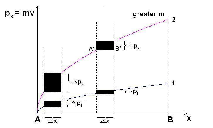
FIGURE \(38.\) The two inevitable curves, stemming from the very definitions of velocity and acceleration, are drawn for two different \(m\) and constant acceleration \(a = \frac{1}{2}m\ s^{-2}\) (Note: constant \(a\) but different \(m\) means that the forces acting, resulting in trajectories \(1\) and \(2\) are different). Same as FIGURE 33 but broken lines drawn to indicate what \(\Delta mv\) would be at a constant \(\Delta x\)
Although the above observation may appear in conflict with what was established from the analysis of FIGURE 37, it actually is not, because the action we talk about here refers to a fixed \(\Delta x\). Therefore, as the motion progresses, it takes less effort, less action as a measure of motion, to traverse the same distance \(\Delta x\), which is in full concordance with FIGURE 37, showing increased action, even when the impulse \(\Delta p\) is kept constant.
Importance of the Law \(v^2=2ax\), eq.(\ref{basiclawofmechanics}), for Motion
When a free body is pushed by a constant force, it is not possible for the body to be at rest. As long as the constant force keeps pushing, the free body will inevitably be in accelerated motion, and, consequently, being in motion, it will inevitably travel through distances, it will inevitably travel through spatial intervals. Motion causes transport through real spatial intervals, ever increasing at that, that transport being inevitably connected with ever increasing change of velocity, until motion ceases at high velocities. These two parameters characterizing the state of the body, spatial displacement and velocity change, are indelibly connected with each other, when the free body experiences motion.
In support of what was just said, one may observe the relationship \(v = \sqrt{x}\) and its graphical representation in FIGURE 38, from which it is obvious that in order to have a non-zero displacement \(x\) in space (or \(\Delta x\), which \(x\) in fact represents), the velocity change \(v\) (or \(\Delta v\), which \(v\) in fact represents) must necessarily be ever increasing; that is, not only is \(v \ne 0\) (\(\Delta v \ne 0\)), but it increases as the distance traveled increases, as long as there is motion, until motion ceases at high velocities.
Now, when looking at FIGURE 38, we must understand that if we truly intend to consider a free body in motion, not a free body at rest, then we must observe a finite, non-zero displacement interval \(\Delta x\) along the x-axis, not just observe one point of the x-axis. Therefore, even if we would claim, in words, that we are observing a free body in motion but, instead, we decide to observe the body at \(\Delta x = 0\), insisting that in this way we are pointing to its concrete single position on the x-axis, we would actually be talking about said body being at rest or at uniform rectilinear (translatory) motion at that certain position on the x-axis at that particular given time \(T\), but will be ignoring the peculiarities of its travel through space under the action of a constant force.
When a free body is pushed by a constant force, it is not possible for the body to be at rest. As long as the constant force keeps pushing, the free body will inevitably be in accelerated motion, and, consequently, being in motion, it will inevitably travel through distances, it will inevitably travel through spatial intervals. Motion causes transport through real spatial intervals, ever increasing at that, that transport being inevitably connected with ever increasing change of velocity, until motion ceases at high velocities. These two parameters characterizing the state of the body, spatial displacement and velocity change, are indelibly connected with each other, when the free body experiences motion.As repeatedly emphasized, motion is more than just a compilation of states of rest. Motion is more than just an assemblage of states of rest. As a matter of fact, if we are oblivious to the fact that the expanded Newton law is an absolute equality, we could, nevertheless, clearly see that mandatory requirement; namely, that there must be a non-zero \(\Delta x\), also in the process of the arrival at that mandatory expansion of Newtons second law, eq.(\ref{FIRSTOCCURRENCEOFrealforce}), if that law is to be written for motion and not just for rest, as it currently exists in standard literature (cf. also here} to see in a general way the signification of rest by Newtons second law, demonstrated by the general equations of mechanics which lead to Newtons second law).
Now, in this book, this more complex characteristic of motion, is confirmed in a most fundamental way, based on absolute truths. It was even shown here that \(F_{real} = ma + \frac{mv^2}{2 x}\) is, in actuality, an expression of the absolute truth \(v^2 = 2ax\)we were able to derive the expression for \(F_{real}\) from \(v^2 = 2ax\) without even suspecting that there is an expression for \(F_{real}\). This derivation proves not only that the expression for \(F_{real}\) is correct, but that the expression for \(F_{real}\) enjoys an absolute validity. Further, the absolute equality \(v^2 = 2ax\) requires us to reckon with the fact, and FIGURE 38 illustrates it, that a finite, non-zero, interval of displacement, is necessarily connected with a finite, non-zero, interval of momentum change. This is another way of restating that displacement in space inevitably leads to change of velocity. Thus, said momentum change indicates that during motion of the body, additional qualitative changes occur, such as change of the energy state of the body. Mere assembly of states of rest does not exhibit that characteristic. Superficially, that fact may not be obvious, and one may be inclined to think that, on the contrary, motion is indeed a compilation of states of rest because, even according to the equation \(v^2 = 2ax\), derived from the definitions of velocity and acceleration, which are absolute truths of physics, a concrete fixed velocity \(v\) corresponds to a concrete, fixed coordinate \(x\), seemingly leaving out the possibility for an uncertainty in determining \(x\) and \(v\).
However, if we really want to observe motion, we must, in addition to the fact that the body will be inevitably at concrete successive positions \(x\) during its motion, that body must also undergo finite displacements \(\Delta x\) from one position to the other, displacements inevitably connected with changes of velocity \(\Delta v\). Furthermore, dont forget that the \(x\) and the \(v\) in \(v^2 = 2ax\) are \(x = x - 0\) and \(v = v - 0\), as was adopted here.
Therefore, when speaking of position and momentum of a free body, having constant force applied to it, we must necessarily talk of intervals, not of concrete individual values of position and momentum.
As an analogy of limited understanding of a concept, consider, for instance, that it is not enough to state that there is a concrete single positive \(v\), corresponding to every single positive \(x\), in order to fully characterize the function \(v = \sqrt{x}\). Disregarding everything else about this function, and insisting that only the mentioned mapping, or response, characterizes the function, is not enough, if we really need to know the properties of the function. If we stop here, considering only the \( x\underbrace{\rightarrow}_\text{ \( \sqrt{ \ \ \ } \)} v \) mapping, and ignore everything else about the function \(v = \sqrt{x}\), claiming that there cannot be anything more about this function, we will be limiting its description. Such description will not be incorrect, but will be limited. The function \(v = \sqrt{x}\) has, for instance, also a non-zero first derivative \(\frac{dv}{dx}\), or, for any mass \(m\), \(\frac{dp}{dx} = \frac{d m\sqrt{x}}{dx} = m\frac{1}{2 \sqrt{x}}\), the existence of which cannot be ignored when characterizing the function more fully.
It is indeed curious that the effect on the physics fundamentals of a basic fact, such as the above (a fact, which demands considering that at the end of interval \(x\), velocity must be non-zero, even if initial velocity is zero), has not been noticed so far, although it is inherent in the very essence of physics, in its very definitions of velocity and acceleration, even the way they are used at present. If one may think that the new ideas expressed herewith might have something to do with the statement that change of \(v\) during motion is unavoidable; that is resolutely not so. The fact that change of velocity \(v\) must requisitely be non-zero when motion takes place, is not something arriving from new views about physics. Far from it. Concerning the new ideas expressed here, these ideas are inherent in physics, they have existed in classical physics, but havent been uncovered. They have remained unnoticed and unexplored even without the mandatory expansion \(F_{real} = ma + \frac{mv^2}{2 x}\) discussed above, eq.(\ref{FIRSTOCCURRENCEOFrealforce}), which introduces the term \(\frac{m v^2}{2x}\) into Newtons second law, to account for the spatial effect of force (cf. here or here), which must be done without a doubt anywayrecall that the known form of Newtons second law expresses change of momentum per unit time, hence, expresses the temporal effect of force only.
There is no substitute for going back to the absolute truths of physics and starting from there, rather than looking for some fantastic, otherworldly, seemingness of new phenomena. If the foundation of creativity in science is not solid; that is, not basing new views in science on fantasies, all else crumbles and what seems like progress is just an illusion.
Based on the above discussion, we can now see how when starting from the solid notions of physics, exemplified by the absolute equality \(v^2 = 2ax\), naturally and inevitably the notions so much fanfared to be distinctly quantum mechanical, turn out to be most decisively belonging to classical mechanics.
The Principle of Least Action Violated During Motion
It is
seen from the equation of classical action \(m \Delta v \Delta x =
\Delta p \Delta x = \Delta w \ne 0\),
eq.(\ref{classicalactiondeltaw}), derived in this book, that the above
mentioned impossibility for a real displacement without non-zero
velocity change, can also be formulated as follows:
It is
not possible for the action to preserve a constant value when a real
change occurs of the generalized impulses and coordinates of a given
mechanical system.
It is known that classical mechanics asserts exactly the opposite: it allows for only such changes of the generalized impulses and coordinates (as a result of the canonical transformations, which we need not discuss herewith), during which action remains unchanged (invariant).
At that, invariance of action is thought (as we see now, thought in error to be invariant!) to comprise one of the most important characteristics of the laws of motion in classical mechanics: \(\delta S = 0\) (principle of stationary action, where in this context \(S\) denotes action.
The invariance of action during displacement (the principle of least action), is an alternative expression of Newtons second law, presented in this way \begin{equation} \Delta w = (F - ma) \Delta x \Delta t = 0. \end{equation} As seen, the above widely recognized law of classical mechanics, still used at present, would be in agreement with the here-discussed inevitable physical fact\(^{92}\), only if \(\Delta w\) is neglected. In other words, only if the motion is so slow, that it is practically a state of rest.
We will note that, under these conditions; namely, the conditions ensuring the state of rest, marking by \(T\) the kinetic energy and by \(v\) the potential energy, the variation of the integral of these two quantities, present under the integral in a peculiar way, is zero; namely, \begin{equation}\label{integralofdeltaaction} \delta \int\limits_{t_0}^{t_1} (T - V) dt = 0, \end{equation} respectively, the integral itself being a constant; namely, \begin{equation}\label{totalactionW} \int\limits_{t_0}^{t_1} (T - V) dt = const. \end{equation} Therefore, taking into account that the kinetic potential of classical mechanics, the Lagrangian \(L = (T - V)\), is constant in force fields, eq.(\ref{integralofdeltaaction}), respectively, eq.(\ref{totalactionW}), is considered a condition that is equated with the \bf principle of conservation of energy \rm \normalfont (CoE) (time-independent).
It follows from the above that the laws of classical mechanics, as they are understood today, which are the basis of the entire classical physics, are in principal contradiction with the absolute fact that no real displacement under the action of a force can occur without change in velocity. According to the classical action inequality \(m \Delta v \Delta x = \Delta p \Delta x = \Delta w \ne 0\), eq.(\ref{classicalactiondeltaw}), derived in this book, the laws of classical mechanics can conform to that impossibility of realizing a real displacement without change of velocity, only as a result of an approximation. Namely, if the value of action \(\Delta w\) of the mechanical system is changed in such a way, as a result of the corresponding change of the generalized impulses and coordinates, that \(\Delta w\) would have a negligibly small value compared to the total action of the system \(W = \int\limits_{t_0}^{t_1} (T - V) dt = const\), eq.(\ref{totalactionW}), and, therefore, we would be able to consider \(\Delta w \approx 0\).
It is seen from FIGURE 33 that the greater the mass and the greater the velocity, the less this \(\Delta w \approx 0\) approximation conforms with reality.
On the contrary, at a sufficiently lower mass and greater force, it is possible to neglect \(W\), respectively \(\Delta w\), and then the motion will acquire the form of FIGURE 44.
The purpose of introducing the Lagrangian \(L = (T - V)\) is to work with energy rather than with force, by having an energy expression, an analog of \(F = ma\)
Therefore, no special attention should be paid to the Lagrangian when one tries to understand the nature of motion, because the Lagrangian suffers from the same deficiencies as the Newton second law, the most significant of which is that the latter is a law of rest, rather than a law of motion. This is also seen from the analysis of Hamilton's equations (cf. here), with which Newtons second law, respectively the Lagrangian, are intimately connected.
Furthermore, the only significant fact regarding the varying of the integral of the Lagrangian, making it equal to zero \begin{equation}\label{secondtimewritingthevaryingofintegral} \delta \int\limits_{t_0}^{t_1} (T - V) dt = 0, \end{equation} is that it is equivalent to \(F = ma\), or if force \(F\) is derived from potential, to \(- \frac{dV}{dx} = m\ddot{x}\), where one dot over \(x\) means a derivative of \(x\) with respect to \(T\); double dot signifies second derivative of \(x\) with respect to \(T\). Only because of this sole goal; namely, to make the integral in eq.(\ref{secondtimewritingthevaryingofintegral}) equivalent to \(F = ma\), is the energy presented in this peculiar way; namely, as \(T - V\). This is the only way for the above integral to arrive at Newtons second law. Therefore, writing the integral is a pure formality, and the analysis of the physical problems, if clarity is to be retained when it comes to motion, should be entirely reverted back to \(F = ma\), not muddled by the introduction of formalities. Thus, if only the temporal aspect of force is sought, the analysis should be based of \(F = ma\). On the other hand, when motion is to be analyzed, the form of the force to take part in the analysis is \(F_{real} = ma + \frac{mv^2}{2x}\). Ergo, analysis of action based on this integral is not needed.
One thing, however, may be useful; namely, to demonstrate that the integral \(\delta \int\limits_{t_0}^{t_1} (T - V) dt = 0\) is indeed equivalent to \(F = ma\). Provided the reluctance in this book to give the impression that mathematics leads physics, giving mundane mathematical detail regarding that analogy may be a slight overkill. However, because for some, this specific \(\left( \delta \int\limits_{t_0}^{t_1} (T - V) dt = 0 \right) \rightarrow (F = ma)\) connection may be felt as central to the argument, we will spend some time on it, in the manner of presenting other trivial points in this book. This would probably allow one to gain better confidence and clarity regarding the contributions herein. Thus, we will now go step by step to show this equivalence between the integral \(\delta \int\limits_{t_0}^{t_1} (T - V) dt = 0\) and Newtons second law.
Proof of the equivalence of \(\delta \int\limits_{t_0}^{t_1} (T - V) dt = 0\) and \(F = ma\)
Understanding the meaning of the symbol \(\Delta\) by using a function as a propTo prove the equivalence between \(F = ma\) and \(\delta \int\limits_{t_0}^{t_1} (T - V) dt = 0\), we will first observe, as an exercise, what the meaning of that peculiar notation \(\delta y(x)\) is, and what it is equal to at the minimum of the function \(y(x)\). We usually perceive \(\delta y(x)\) as only the change in \(y(x)\), unlike the derivative of \(y(x)\) with respect to \(x\); namely, \(\frac{dy}{dx}\). In other words, \(\delta y\) is \(dy\) of sorts, without treating \(dy\) as the differential; that is, as the main (principal) part of the very small change of \(y(x)\); namely, \(\frac{dy}{dx}dx\), but considering the entire infinitesimal change of \(y(x)\).
In this case, however, we will express \(\delta y\) with the help of the small quantity \(\Delta x\). Thus, \(\delta y = y(x + \delta x) - y(x)\). Now, we assert that, if the minimum of the function \(y(x)\) is at point \(x\), then we will have \begin{equation}\label{varyingyx} \scriptsize \delta y = y(x + \delta x) - y(x) = 0 \end{equation} to first order of approximation (linear) in this variation \(\Delta x\) of the independent variable.
The above criterion, eq.(\ref{varyingyx}), for the minimum of \(y(x)\) at point \(x\) does not seem immediately obvious, so, let us see why this is so. To do that let us first apply a linear Taylor approximation of the first term on the right side of the equality, eq.(\ref{varyingyx}), the function \(y\) of the argument \((x + \delta x)\). We have, \(y(x + \delta x) \approx y(x) + \frac{\partial y}{\partial x} \delta x\), retaining only the first order term in \(\delta x\). Therefore, substituting it in eq.(\ref{varyingyx}) for \(y(x + \delta x)\) we get \begin{equation*} \scriptsize \delta y = \require{cancel}\bcancel{y(x)} + \frac{\partial y}{\partial x} \delta x - \require{cancel}\bcancel{y(x)} \end{equation*} \begin{equation}\label{deltayaftercancellation} \scriptsize \delta y = \frac{\partial y}{\partial x} \delta x. \end{equation} In this way, we expressed the object peculiarly denoted by \(\delta y(x)\), whose meaning is unknown to us, in terms of something; that is, in terms of \(\frac{\partial y}{\partial x}\), which, as a mathematical object, we already know from calculus. This is the so-called first (partial) derivative of \(y(x)\) with respect to \(x\). Furthermore, we also know from calculus that if the function \(y(x)\) has a minimum at point \(x\), then \(\frac{\partial y}{\partial x}\) must be \(0\). Therefore, eq.(\ref{deltayaftercancellation}) must be \begin{equation} \scriptsize \delta y = \frac{\partial y}{\partial x} \delta x = 0. \end{equation} This is how we proved that, indeed, when the function \(y(x)\) has a minimum, its variation \(\delta y(x)\) must be 0.
What we did so far is to explain what this peculiar symbol \(\Delta\) is and does when it concerns a function. This knowledge we are now going to use with the functional \(\int\limits_{t_0}^{t_1} (T - V) dt\).
Using the above-illustrated meaning of the symbol \(\Delta\) on a functionalWe are now going to assert that the \(\Delta\) of the functional in question will have minimum when that \(\delta \int\limits_{t_0}^{t_1} (T - V) dt\) is equal to zero. Let us denote the above functional, comprising action, by \(S[x(t)] = \int\limits_{t_0}^{t_1} (T - V) dt\) and see what \(\delta S[x(t)] = \delta\int\limits_{t_0}^{t_1} (T - V) dt = 0\) is. We kind of assume, judging from what we said when considering \(\delta y(x)\), whereby we demonstrated that the \(\delta y(x) = 0\) guarantees to first order of approximation in \(\Delta x\), that \(y(x)\) has a minimum at point \(x\), that this procedure concerning \(\delta y(x)\) will guarantee us that \(\delta S[x(t)] = \delta\int\limits_{t_0}^{t_1} (T - V) dt = 0\) signifies the minimum of the functional \(S[x(t)] = \delta\int\limits_{t_0}^{t_1} (T - V) dt\). However, what we are really interested in, is what this \(\delta S[x(t)] = \delta\int\limits_{t_0}^{t_1} (T - V) dt = 0\) is going to be equal to (HINT: With the risk to ruin the fun, we will jump the gun now and will give away the outcomethe mathematical object, or expression, \(\delta S[x(t)] = \delta\int\limits_{t_0}^{t_1} (T - V) dt = 0\) is nothing other than another way of expressing Newtons second law, \(- \frac{\partial V}{\partial x} = m\ddot{x}\)).
Despite the above premature revelation, why not enjoy the entire road of reaching that conclusion of equivalency. For this reason, we apply the same approach as the approach we applied when discussing the variation \(\Delta\) of the function \(y(x)\). Thus, we form \begin{equation} \scriptsize \delta S = S[x(t) + \delta x(t)] - S[x(t)], \end{equation} and require, by analogy with the varying \(\delta y(x)\) of a function and requiring that \(\delta y(x) = 0\), that the above \(\delta S\) be \(0\) to first order in the variation \(\delta x(t)\).
Now, we can present the above expression containing the integral \(\delta \int\limits_{t_0}^{t_1} (T - V) dt = 0\) explicitly by writing \(\frac{1}{2}mv^2 = \frac{1}{2}m\dot{x}^2\), substituting for \(T\), and \(V(x)\) substituting for \(v\), resulting in \begin{equation} \scriptsize S[x(t)] = \int\limits_{t_0}^{t_1} \left(\frac{1}{2}m\dot{x}^2 - V(x)\right) dt \end{equation} and \begin{equation}\label{equationtobeexpanded} \scriptsize S[x(t) + \delta x(t)] = \int\limits_{t_0}^{t_1} \left( \frac{1}{2}m\left(\dot{x} + \delta \dot{x}\right)^2 - V(x + \delta x)\right) dt. \end{equation} Now, we expand \(\frac{1}{2}m\left(\dot{x} + \delta \dot{x}\right)^2\) in eq.(\ref{equationtobeexpanded}), which gives \(\frac{1}{2}m\dot{x}^2 + \require{cancel}\bcancel{2}\frac{1}{\require{cancel}\bcancel{2}} m\dot{x}\delta \dot{x}+ \cancel{\delta \dot{x}^2}\), canceling \(\delta \dot{x}^2\) as negligibly small (because we are working only to first order in \(\delta \dot{x}\)), and also, in the same eq.(\ref{equationtobeexpanded}), linearize \(V(x + \delta x)\) to first order in the variation \(\delta x(t)\), as \(V(x ) + \frac{\partial V}{\partial x} \delta x\), obtaining finally \(S[x(t) + \delta x(t)] = \int\limits_{t_0}^{t_1} \left( \frac{1}{2}m\dot{x}^2 + m\dot{x}\delta \dot{x} - V(x ) - \frac{\partial V}{\partial x} \delta x\right) dt\). Now we are ready to form the difference \(S[x(t) + \delta x(t)] - S[x(t)]\), which becomes \begin{equation*} \scriptsize \int\limits_{t_0}^{t_1} \left( \frac{1}{2}m\dot{x}^2 + m\dot{x}\delta \dot{x} - V(x ) - \frac{\partial V}{\partial x} \delta x - \left( \frac{1}{2}m\dot{x}^2 - V(x) \right)\right) dt = \end{equation*} \begin{equation*} \scriptsize \int\limits_{t_0}^{t_1} \left( \require{cancel}\bcancel{\frac{1}{2}m\dot{x}^2 }+ m\dot{x}\delta \dot{x} \require{cancel}\bcancel{ - V(x )} - \frac{\partial V}{\partial x} \delta x \require{cancel}\bcancel{ - \frac{1}{2}m\dot{x}^2} \require{cancel}\bcancel{ + V(x)} \right) dt = \end{equation*} \begin{equation}\label{interimresultfordeltaS} \scriptsize \int\limits_{t_0}^{t_1} \left( m\dot{x}\delta \dot{x} - \frac{\partial V}{\partial x} \delta x \right) dt. \end{equation} Eq.(\ref{interimresultfordeltaS}) contains \(\delta \dot{x}\), so we need to substitute it somehow by \(\delta{x}\), in order to have everything proportional to \(\delta{x}\) itself. Therefore, we observe that \begin{equation*} \scriptsize \frac{d}{dt} (m \dot{x} \delta{x}) = m\ddot{x}\delta x + m\dot{x} \delta \dot{x} \end{equation*} or, reordered \begin{equation*} \scriptsize m\dot{x} \delta \dot{x} = \frac{d}{dt} (m \dot{x} \delta{x}) - m\ddot{x}\delta x. \end{equation*} The latter is substituted in eq.(\ref{interimresultfordeltaS}) \begin{equation*} \scriptsize \int\limits_{t_0}^{t_1} \left( \frac{d}{dt} (m \dot{x} \delta{x}) - m\ddot{x}\delta x - \frac{\partial V}{\partial x} \delta x \right) dt = \end{equation*} \begin{equation*} \scriptsize \int\limits_{t_0}^{t_1} \left(\frac{d}{dt} (m \dot{x} \delta{x})\right) dt - \int\limits_{t_0}^{t_1}\left( m\ddot{x} + \frac{\partial V}{\partial x}\right)\delta x dt = \end{equation*} \begin{equation*} \scriptsize \int\limits_{t_0}^{t_1} d (m \dot{x} \delta{x}) - \int\limits_{t_0}^{t_1}\left( m\ddot{x} + \frac{\partial V}{\partial x}\right)\delta x dt = \end{equation*} \begin{equation*} \scriptsize m \dot{x} \delta{x}\Big|_{t_0}^{t_1} - \int\limits_{t_0}^{t_1}\left( m\ddot{x} + \frac{\partial V}{\partial x}\right)\delta x dt. \end{equation*} However, the variations at the ends of the trajectories, which are constant, are \(0\). Therefore, \(\delta x(t_0) = 0 = \delta x(t_1)\). Thus, the first term is \(0\) and we get \begin{equation}\label{integralcontainingNewtonslaw} \scriptsize - \int\limits_{t_0}^{t_1}\left( m\ddot{x} + \frac{\partial V}{\partial x}\right)\delta x dt = 0. \end{equation} This implies \(\left( m\ddot{x} + \frac{\partial V}{\partial x}\right) = 0\), because \(\Delta x\), albeit very small, is a finite non-zero quantity, or, reordered, it finally yields \begin{equation} \scriptsize - \frac{\partial V}{\partial x} = m\ddot{x}, \end{equation} which is Newtons second law. This accomplishes our task aimed at proving equivalency between \(F = ma\) and \(\delta \int\limits_{t_0}^{t_1} (T - V) dt = 0\).
Of course, the above discussion may be generalized by obtaining \(\frac{d}{dt}\frac{\partial L}{\partial \dot{x_i}} - \frac{\partial L}{\partial x_i} = 0\), but for the purposes of our study what was derived so far suffices.
The curious, however, may observe that \begin{equation} \scriptsize \delta S = \int\limits_{t_0}^{t_1} \delta L(x, \dot{x})dt, \end{equation} and, since, in our case, \(L = T - V = \frac{1}{2}m\dot{x}^2 - V(x)\), we have \begin{equation}\label{minusdVdx} \scriptsize \frac{\partial L}{\partial x} = - \frac{dV}{dx}, \end{equation} because we are taking partial derivative with respect to \(x\), not with respect to \(\dot{x}\). Thus, the partial derivative with respect to \(x\) of the first term \(\frac{1}{2}m\dot{x}^2\) in the equation for \(L\); namely, \(L = T - V = \frac{1}{2}m\dot{x}^2 - V(x)\), is zero.
On the other hand, we see that the first term on the right of \(L = T - V = \frac{1}{2}m\dot{x}^2 - V(x)\) contains \(\dot{x}\), but does not contain \(x\), the first derivative of \(L\), this time with respect to \(\dot{x}\), will be \begin{equation}\label{firstderivativewrtofmdoubledot} \scriptsize \frac{d}{dt} \left( \frac{\partial L}{\partial \dot{x}} \right) = \frac{d}{dt} (m \dot{x}) = m \ddot{x}. \end{equation} Therefore, summing up eq.(\ref{minusdVdx}) and eq.(\ref{firstderivativewrtofmdoubledot}), we get \begin{equation} \scriptsize \frac{\partial L}{\partial x} - \frac{d}{dt} \left( \frac{\partial L}{\partial \dot{x}} \right) = - \left( m \ddot{x} + \frac{dV}{dx} \right). \end{equation} This means that the expression on the left of the equality sign is the same as the expression in the parentheses in eq.(\ref{integralcontainingNewtonslaw}). Therefore, we may substitute \(\frac{\partial L}{\partial x} - \frac{d}{dt} \left( \frac{\partial L}{\partial \dot{x}} \right)\) for \(- \left( m \ddot{x} + \frac{dV}{dx} \right)\) in that equation, eq.(\ref{integralcontainingNewtonslaw}), and get \begin{equation} \scriptsize \delta S = \int\limits_{t_0}^{t_1} \delta L(x, \dot{x})dt = \int\limits_{t_0}^{t_1} \frac{\partial L}{\partial x} - \frac{d}{dt} \left( \frac{\partial L}{\partial \dot{x}} \right) \delta x dt = 0. \end{equation} The above integral is \(0\) when \begin{equation}\label{EulerLagrangeequation} \scriptsize \frac{\partial L}{\partial x} - \frac{d}{dt} \left( \frac{\partial L}{\partial \dot{x}} \right) = 0, \end{equation} because, again, \(\Delta x\) is not zero. Eq.(\ref{EulerLagrangeequation}) is known as Euler-Lagrange equation, sometimes written as \(\frac{\partial L}{\partial q_i} - \frac{d}{dt} \left( \frac{\partial L}{\partial \dot{q_i}} \right) = 0\), where \(q\) is generalized coordinate. The second-order Euler-Lagrange equation can be expressed as two first-order Hamiltons equations, which simplifies calculations. However, what is especially important in the discussed context is that Hamiltons equations are clearly expressing the state of rest of a system (cf. here), which means that, along this line of reasoning, also Euler-Lagrange equation, as well as Newtons second law derived from them, are also equations of rest. Thus, one cannot help but notice how intertwined all these seemingly unconnected equations are, all of them signifying one staterest. On the other hand, analysis of motion can take place only along a different cogitation line; namely, that line of reasoning beginning with the most fundamental equation of mechanics (dynamics), which in this book is always cited as \(v^2 = 2ax\).
Mathematics vs. physics
We were considering a body (in the discussion we just ended, it was a charged particle whereby Newtons second law \(F = ma\) has the form \(- \frac{\partial V}{\partial x} = m\ddot{x}\)) moving along the x-axis under the influence of some potential and wrote a peculiar expression, \(\left( \delta \int\limits_{t_0}^{t_1} (T - V) dt = 0 \right)\), involving the kinetic and potential energy of the charged particle. The expression was specially designed, purely formally, in such a way that it would be equivalent to Newtons second law.
The above was another example (along with cases such as those and those) of using a mathematical equation in the process of illustrating or aiding in solving of physical problems. In doing so, as remarked also in the mentioned earlier pages, we must not overstep the boundaries of physics and get carried away by endowing mathematical constructs with non-existing physical meaning. Thus, in the observed case, Newtons second law, especially its expanded form \(F_{real} = ma + \frac{mv^2}{2x}\), to say nothing of the absolute equality \(v^2 = 2ax\), from which the expanded Newtons second law evolves, has the leading role in determining physical conclusions. Therefore, any physical conclusion that may occur to us, as if arriving from a mathematical construct, must be checked, in principle, against the physics of the situation. In this particular instance (considering the integral \(\left( \delta \int\limits_{t_0}^{t_1} (T - V) dt = 0 \right)\)), specifically against the firm physical content of Newtons second lawthe most important as physical content, in this case being the fact that Newtons second law is an equation of rest, not of motion, as was discussed earlier.
As is discussed above, \(F = ma\) is correct but only in a limited sense, considering only the temporal characteristic (lacking the spatial characteristic) of force. This fact cannot be anything but reflected in the above-observed integral \(\delta \int\limits_{t_0}^{t_1} (T - V) dt = 0\), eq.(\ref{integralofdeltaaction}), because that integral is equivalent to \(F = ma\), as was demonstrated.
Notice, \(F = ma\) is an equation of rest (cf. as seen), despite the fact that even at \(a = const\), the quantity \(\frac{dx}{dt}\), which is velocity \(v\) and which participates in the non-zero acceleration, is not 0 in the expression \(F = ma\). So, the velocity \(v\) is not equal to 0, and yet the body at hand is at rest because of the content of Newtons second law in the form it exists in the standard texts.
So, when a body (in this case a charged particle) is considered, moving along the x-axis under the influence of some potential, then we should not contemplate the known force \(F\), but should contemplate only the operative part of \(F_{real}\), comprising exactly half of \(F_{real}\) (cf. eq.(\ref{F12Freal}), as well as keep in mind the discussion on interpretation of \(F_{real} = 2ma\) here.
A consideration may emerge now, pertaining to the equivalence between the equation \(\delta \int\limits_{t_0}^{t_1} (T - V) dt = 0\), and \(\left( - \frac{\partial V}{\partial x} = m\ddot{x}\right)\), the latter equation \(\left( - \frac{\partial V}{\partial x} = m\ddot{x}\right)\) having, on the face of it, the exact appearance of the known Newton second law, written usually as \(F = ma\). In actuality, the motion-causing-force is not that force \(F\) seen in the Newtons second law floating in the mainstream, but, when it comes to the force causing motion, that force is a spin-off of the force \(F_{real}\). In fact, that motion-causing-force is exactly half of \(F_{real}\). \(F_{real}\) has the content \(F_{real} = ma + \frac{mv^2}{2x}\), respectively, \(F_{real} = 2ma = 2F\). Thus, the force \(F\) seen in the standard literature, is the first \(F\) in this \(F_{real} = 2F\) expression, while the second \(F\) in this \(F_{real} = 2F\) expression, is the motion-causing-force.
Such question finds its answer by one, again, recalling that the usual \(F = ma\), present in the standard literature, is an equation of rest (cf. here), and if that were indeed the force about which we express interest; that is, the force causing real, operative motion, then the body would not have moved from its initial position. We would be disappointed since there would be no motion. There would have been no trajectory at all that might have been ascribed to it. The traversing of the trajectory from its beginning at \(t_0\) to its end at \(t_1\), along which the body has traveled from point \(x_0\) to point \(x_1\), is due to the second part \(F\) of the real force \(F_{real} = 2F\), which happens to be exactly equal in form and magnitude to the non-operative part of the force; namely, \(F\), comprising the first part, first half of force \(F_{real} = 2F\), and the discussion on the interpretation of \(F_{real} = 2ma\).
Furthermore, as was seen above, no matter what interpretations one may come up with regarding the equivalent forms of that equation, the equation for \(F_{real} = ma + \frac{mv^2}{2x}\) is an absolute equality, which arrives from the absolute equality \(v^2 = 2ax\) (cf. here and here. Therefore, everything again boils down to that most fundamental, absolute equality of mechanics, \(v^2 = 2ax\).
Having that in mind, it stands to reason that no varying and equating to zero of an integral of the sort of \(\int\limits_{t_0}^{t_1} (T - V) dt\) is even needed, in order to know what trajectory the body under consideration should follow. The only possible trajectory for a free body driven by a constant force, is given by the absolute equality \(v^2 = 2ax\). Some may venture to say that strictly speaking trajectory is \(x = f(t)\). However, expressing that is straightforward from the conditions under which \(v^2 = 2ax\) is derived.
In other words, we have to realize what this equivalence, which we proved, between \(\delta \int\limits_{t_0}^{t_1} (T - V) dt = 0\) and, what comes out as, \(F = ma\), really means.
In
order to understand what it all means, we have to consider the
simplest possible case, such as the case we are discussing
herewithmotion of a free body impelled by a constant force along the
x-axis. Accidentally, in such a case, it must be clear that the
equivalence of the integral \(\delta \int\limits_{t_0}^{t_1} (T - V)
dt = 0\), eq.(\ref{integralofdeltaaction}), and the Newtons second
law is only when Newtons second law is expressed as the limited law
\(F = ma\), and is not in its expanded form \(F_{real} = ma +
\frac{mv^2}{2x}\).
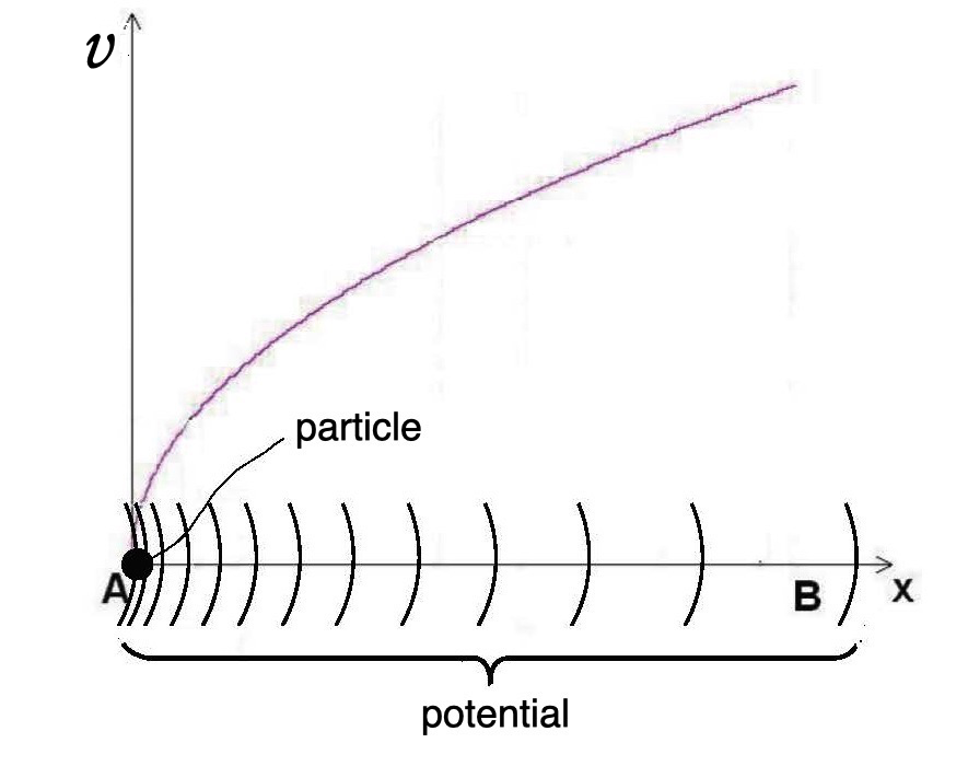
FIGURE \(39.\) Velocity \(v\) as a function of displacement \(\Delta x = x - 0\) for a particle of unit mass acted upon by a constant force. The constant force is ensured by a constant gradient \(\left( -\frac{dV}{dx} \right)\), along the direction of the particles motion of a linearly decreasing potential (hence, the minus sign in the formula, reflecting the fact that the potential decreases as \(x\) increases), following the positive values of x-axis. The linearly decreasing potential is depicted by arcs outstanding at greater and greater distances along the x-axis, as the potential gets lower. Recall, we need a potential only for the purposes of forming the variation of the functional \(\delta \int\limits_{t_0}^{t_1} (T - V) dt = 0\). Otherwise, one wont be able to show that said integral is equivalent to \(- \frac{dV}{dx} = m\ddot{x}\), which usually is written as \(F = ma\).
Thus, it is true that conservation of energy (CoE) is obeyed at every point of the trajectorythe motion of the charged particle in the direction opposite to the increasing potential (cf. FIGURE 39)imagine a waterfall, whereby the water is falling from high to low altitude, in a direction opposite to the direction of the increase of heightthe combined kinetic and potential energy, which the charged particle has along the horizontal AB trajectory will remain constant, despite the changing proportions amongst potential and kinetic energy. At every point along AB trajectory the charged particle has ever decreasing potential energy with respect to the potential at point B, while the kinetic energy experiences increase.
However,
it is not the integral and its minimization, but the absolute equality
\(v^2 = 2ax\) which will determine the one and only one
possible trajectory, although at the end of the trajectory, just like
the integral \(\int\limits_{t_0}^{t_1} (T - V) dt = const\), the
integral \(W = \int\limits_{x_0}^{x_1} m\dot{x}dx\) will be
represented by a given constant, for the here-considered unit mass
\(m\).
Further illustrationrelations showing non-constancy of action
The
above observation for the uniqueness and constancy of the integral
\(\int\limits_A^B m\dot{x}dx\) along the entire path AB in FIGURE
40 for a free body of mass \(m\) and constant acceleration \(a =
\frac{1}{2}\), may be applied to every segment, or call it, sub-path,
say AA\('\) or A\('\)A\(''\) and so on, of that path AB.
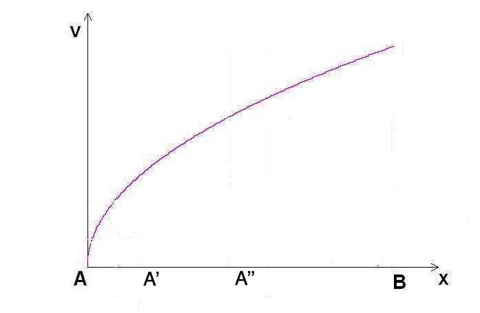
FIGURE \(40.\) Velocity as a function of displacement for a body of mass \(m\) and non-negligible constant acceleration, say, \(a = \frac{1}{2}\). Sub-paths AA\('\), AA\(''\) ... of the main AB path are also indicated.
In other words, we will have, say, \( \int\limits_{A}^{A'} m\dot{x}dx \), \(\int\limits_{A'}^{A''} m\dot{x}dx\), \( \int\limits_{A}^{A''} m\dot{x}dx \) or \(\int\limits_{A''}^{B} m\dot{x}dx, \dots\), which will all be constant in this given case, but of varying value. In other words, along the way from A to B, characterized by the action of constant value \(\int\limits_A^B m\dot{x}dx\) at the case at hand, as well as in each case similar to the case at hand, but each one case of operative motion having its own characteristic constant. The motion of the particular observed body is characterized by a constant overall action along the AB trajectory, but consisting of sub-paths, say, \(\int\limits_{A}^{A'} m\dot{x}dx\) and so on, each one having different definite constant value of its own. As said, no minimization of the integral along different paths between the end points A and B is necessary, in order to establish the constant path along the minimum of the functional (the integral) from A to B, as classical mechanics requires thus far. The value of the integral between A and B is still only one constant value but that value is the only one possible value.
To make the above a little more visual, let us take a numerical example. Thus, let our free body, having constant acceleration \(a = \frac{1}{2}\) and velocity \(v = \sqrt{x}\), traverse a trajectory spanning from \(x = 0\) to \(x = 10\). Then, consider that the interval of \(x\) for which we are going to calculate the individual \(\Delta w\) along the trajectory is constant and is equal to \(\Delta x = 1\). Under these conditions, the partial action \( \Delta w = \Delta p \Delta x = m\Delta v \Delta x = m.(v(x) - v(x - 1) \).
\( \Delta x = m \left(\sqrt{x} - \sqrt{x - \Delta x}\right) \Delta x \) along the spatial coordinate \(x\) obtains the form \( \Delta w = m \left(\sqrt{x} - \sqrt{x - 1}\right) 1 \).
We may now illustrate that action does not remain constant during the motion from the initial point A to the final point B of the trajectory, by plotting that \(\Delta w = m \left(y(x) - y(x - 1)\right)\Delta x = m \left(\sqrt{x} - \sqrt{x - 1}\right) 1\) against \(x\) for some value of \(m\), say, \(m = 1\), FIGURE 41.
However, if we want to see what the change of the action \(\Delta w\) looks like as a function of \(x\), independent of mass \(m\), we may divide \(\Delta w = m \left(\sqrt{x} - \sqrt{x - 1}\right)\) by the overall action \(W = m\int\limits_{0}^{10} v(x) dx = m\int\limits_{0}^{10} \sqrt(x) dx\); that is, \( \frac{\require{cancel}\bcancel{m} \left(\sqrt{x} - \sqrt{x - 1}\right)}{ \require{cancel}\bcancel{m}\int\limits_{0}^{10} \sqrt(x) dx}\), by calculating the value of that overall action \(W = m\int\limits_0^{10} \sqrt{x}dx = m\frac{2x^{\frac{3}{2}}}{3}\Big|_0^{10} \approx m21\) for the whole span \([0,10]\) of \(x\), and as a result forming the quotient \(\frac{\require{cancel}\bcancel{m} (\sqrt{x} - \sqrt{x - 1})}{\require{cancel}\bcancel{m}21}\). We can, then, plot it against \(x\), spanning from \(x_1 = 0\) to \(x_2 = 10\), FIGURE 42.
Alternatively, we can eliminate mass \(m\) as \(W\) increases with
\(x\) (not, as in FIGURE
42, whereby \(W\) was fixed as \(m21\) for the entire \([0,10]\)
span of \(x\), encompassing the entire AB trajectory) spanning from
\(x_1 = 0\) to \(x_2 = 10\), together with the increase of \(m
(\sqrt{x} - \sqrt{x - 1})\) with \(x\)mass \(m\) cancels outFIGURE
43.
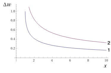
FIGURE \(41.\) Plot of \(\Delta w\) as a function of \(x\). This graph shows that action changes, decreasing its value, during the travel across the trajectory of the free body impelled by a constant force. The graph in this figure depends on the masscurve 1, mass \(m = 1\), curve 2, mass \(m = 2\). Use Wolfram Alpha code to plot it on the net: plot (sqrt(x)- sqrt(x-1)), (2(sqrt(x)- sqrt(x-1))) for x = 0 to x = 10.
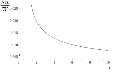
FIGURE \(42.\) \(\frac{\Delta w}{W}\) as a function of \(x\), where \(W = m21\) is calculated for the entire \([0.10]\) span of \(x\). Wolfram Alpha code: plot (sqrt(x) - sqrt(x-1))/(int\text{\_}0\^{}10 sqrt{x} dx) for x = 0 to x = 10.
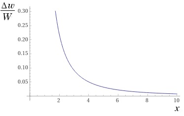
FIGURE \(43.\) \(\frac{\Delta w}{W}\) as a function of \(x\), whereby \(W\) is calculated consecutively for each \(x\), as \(x\) grows. Wolfram Alpha code: plot (sqrt(x) - sqrt(x-1))/(int\text{\_}0\^{}x sqrt{x} dx) for x = 0 to x = 10.
It is hard to say which one of the three figures shown is preferable, but that doesnt even matter because we are interested only in the trend the curves display, which demonstrates that the value of action decreases with \(x\) along the trajectory of a free body propelled by a constant force for the entire path of the trajectory, until action vanishes asymptotically, as \(x\) increases further, beyond the trajectory \([0,10]\) of \(x\) in this example, the operative motion gradually turning into non-operative uniform translatory motion.
Of course, aside from FIGURE 42 and FIGURE 43 both showing asymptotic decline of acton independent of mass \(m\), understandably, the curve seen in FIGURE 43 goes down faster because the ever decreasing \(\Delta w\) is being divided by an ever increasing \(W\). The degree of sloping down of the curve in FIGURE 42 is less because the decreasing value of \(\Delta w\) is divided by a constant, 21, and that makes the run of the curve in FIGURE 42 exactly the same as the run of the curve in FIGURE 41, save the fact that, unlike FIGURE 41, the graph in FIGURE 42 is valid for any mass \(m\).
However, the fact that the elementary quantum of action \(\Delta w\) has the form of a curve dropping fast asymptotically to zero with \(x\), transforming operative motion into non-operative uniform translatory motion, akin to rest, we already knew from the earlier analysis. The above figures were shown just for fun. The effect seen in FIGURE 41FIGURE 43 reproduces the effect for a given \(\Delta x\), seen in FIGURE 38. As was discussed under FIGURE 38, the falling value of action, respectively, the \(\frac{\Delta w}{W}\) ratio, as the value of \(x\) increases, indicates that the more the free body is removed from its position of rest (\(x = 0\)) by the applied constant force, the easier it is (the action becomes lower) for that body to traverse the same distance \(\Delta x\). This observation resulting from Figure 41FIGURE 43 confirms the conclusion drawn from FIGURE 38the more removed from its position of rest, \(x = 0\), the closer the free body approaches uniform translatory motion, which means the more the operative motion wanes.
In other words, in the example given, exemplifying all cases of operative motion, the elementary quantum of action \(\Delta w\) is not constant throughout the trajectory, as classical mechanics would (mistakenly!) have it, at present.
Action when moving the body between two positions of rest
Observe
the displacement of a body from a spatial point \(a\), where the body
has velocity \(v = 0\), to another spatial point \(B\), where the
body's velocity is also \(v = 0\), illustrated in FIGURE
44. It is seen from FIGURE 44, that,
if the body is passing from one state of rest into another state of
rest, the impossibility for a real transport of the free body between
points A and B to occur without change of velocity, is true even in
absence of a force field existing prior to the transportation.
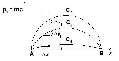
FIGURE \(44.\) Family of some possible trajectories, necessarily curvilinear, to move a body by operative motion from point A to point B. True motion, operative motion, of the body along the straight line trajectory AB, or any other trajectory parallel to AB, is impossible. The body traverses the straight line trajectory AB, or any other trajectory parallel to AB, with uniform translatory motion which is akin to rest. Such motion is non-operative, it is not motion at all.
Of course, for that displacement, a displacement taking place between the two states of rest, to occur, force is also applied, variable at that. Therefore, once force is involved, real displacement due to real, operative, motion, cannot occur without change of velocity and doing work. According to the here-discussed impossibility to have a real motion without velocity change, any of the non-linear phase trajectories (change of velocity with position) \(AC_1B\), \(AC_2B\), \(AC_3B\) ... is possible because velocity changes, but it is never possible to have real, operative, motion along the linear phase trajectory \(AB\), despite the fact that the body is displaced from A to B. Mere displacement, without the qualitative change epitomized by change of velocity, is not real motion, but such a state, called uniform translatory motion, is akin to rest. The qualitative change, characterized by change of velocity, is crucial for the displacement to be considered a result of real, operative, motion.
It is also to be noted, that the equality \(m \Delta v \Delta x = \Delta p \Delta x = \Delta w \ne 0\), eq.(\ref{classicalactiondeltaw}), which was observed so far only for a constant force, applies in this instance, concerning varying force, as well.
Uniform linear (translatory) motion
It is seen from FIGURE 44 that the equality \(\Delta p \Delta x = \Delta w = 0\) is only observed in the case of uniform linear (also known as uniform rectilinear, or uniform translatory) motion (the phase trajectory along the horizontal section \(AB\), or along any path parallel to AB, for that matter). In other words, when the acceleration is zero, the dynamic laws of what is now considered as classical mechanics, are valid with theoretical exactness only in the case of uniform linear (translatory) motion\(^{93}\).
The Uncertainty Principle in Quantum Mechanics Finds its Real Meaning in the Classical Relation \(\Delta x \Delta p = \Delta w \ne 0\)
It was mentioned here, that the inequality \(m \Delta v \Delta x = \Delta p \Delta x = \Delta w \ne 0\), eq.(\ref{classicalactiondeltaw}), is also an expression of the classical uncertainty relation.
In this section, we will once again observe the quantities \(\Delta x\) and \(\Delta p\), as quantities representing the uncertainties, \(\Delta x\) and \(\Delta p\), of measuring \(x\) and \(p\) in classical mechanics, and will compare their product with what is known as the uncertainty principle in quantum mechanics. Of course, we are doing this comparison with a claimed outcome from quantum mechanics only as an exercise, for the sake of discussion. In truth, we must not deal with any purported conclusion stemming from the non-scientific quantum mechanics, the non-scientificity of the latter following from the ample arguments given in this book. This must be kept in mind anytime the term quantum mechanics is brought into the present narrative.
As far as classically measuring \(x\) and \(p\) goes, when a free body is in motion under a constant force; that is, when a free body is in operative motion, these two parameters cannot be measured exactly at the same time. It is impossible to have the uncertainties of their respective measurements simultaneously be \(\Delta x = 0\) and \(\Delta p = 0\). In other words, in classical mechanics, as in what is purported to occur in quantum mechanics, when measuring the coordinate exactly; that is, when \(\Delta x = 0\), the measurement of the momentum \(p\) is infinitely inexact, that is, \(\Delta p \rightarrow \infty\). Again, we are talking about operative motion, dont forget.
Classically, this is seen at once from the expression \(m \Delta v \Delta x = \Delta p \Delta x = \Delta w \ne 0\), eq.(\ref{classicalactiondeltaw}), which was discussed above as action. Indeed, it is seen at once from \(m \Delta v \Delta x = \Delta p \Delta x = \Delta w \ne 0\), eq.(\ref{classicalactiondeltaw}), reordered as \begin{equation} \Delta p = \frac{\Delta w}{\Delta x}, \end{equation} that if the uncertainty \(\Delta x\) in measuring \(x\), is zero; that is, if \(x\) is measured exactly, then the uncertainty \(\Delta p\) in measuring \(p\), is infinity. It is seen, however, even numerically (cf. here, that even if \(\Delta p\) and \(\Delta x\) are very small, say, \(\frac{dp}{dx}\), none of them can be zero if there is motion. When there is real, operative, motion we see that no matter how tiny the non-zero \(dw\) is, \(dw\) being equal to the product \(dxdp\) of the two uncertainties, nevertheless \(dp\) will be infinity if \(x\) is known exactly; that is, if \(dx\) is zero. This is immediately seen from \(dp = \frac{dw}{dx}\), whereby the infinite certainty in knowing \(x\), \(dx = 0\), causes \(dp\) to become \(\infty\); that is, causes \(p\) to become infinitely uncertain, rather, undefined in view of the forbiddance of division by \(0\) or by \(\infty\).
The hitherto unrecognized genuine classical uncertainty obviously suggests discontinuity (quantumness), the same way quantum mechanics suggests discontinuity (quantum character) because of the claimed presence of the uncertainty principle, in contrast to the presumed continuity, expressed by\(^{94}\) \begin{equation} \label{uncertainyrelationsatuniformmotion} \Delta x \Delta p_x = \Delta w = 0, \end{equation} by what is known at present as classical physics. However, as already mentioned, when contemplating the principle of inevitable non-zero velocity change during real displacement of a free body under the action of a constant force; that is, when contemplating real, operative motion, it is important to realize that, also when classical uncertainty principle is had in mind, the equality, eq.(\ref{uncertainyrelationsatuniformmotion}), is only true in the case of rest or in the case akin to rest, known as uniform linear (translatory) motion only (motion along horizontal phase trajectories, parallel to the x-axis of FIGURE 33.
It is also important to notice that when there is motion of a free body; that is, when the free body experiences acceleration as a result of a constant force impressed on it, uncertainty relations arise in classical physics only because of the mere fact that \(\Delta p_x \Delta x = \Delta w \ne 0\), not because the non-zero value of \(\Delta w\) is equal to or greater than some given fixed non-zero value (\(\Delta x \Delta p_x \geq \frac {\hbar} {2}\)), as it purportedly is in quantum mechanics.
Incidentally, even classically, in the particular phenomenon of blackbody radiation, which does not concern motion of a free body, but relates to electromagnetic phenomena, the value of \(\Delta w\), in this particular case of blackbody radiation, is equal to \(\mathscr{h}\,\). The reason for that is that the average quanta of exchanging energy, correctly derived, at that classically, which the explanation of blackbody radiation is based on, are characterized by this minimum amount of action. The concrete value of \(\mathscr{h}\,\) is determined from experimental curves such as those found by Lummer and Pringsheim\(^{24}\), the way the value of constant \(h\) is found in \(\S11\) and \(\S12\) of Plancks paper\(^{1}\). The numerical coincidence of the \(\mathscr{h}\,\) and \(h\) value is due to the fact that Plancks and C. I. Noninskis curve has the same shape, reproducing the shape of the experimentally found curve. The difference is that C. I. Noninskis curve is derived, classically at that, while Plancks curve is a result of finagling with formulae until the right shape came out, which is a process similar to curve-fitting, implying the involvement of no theory at all.
It should be noted also that the uncertainty principle in quantum mechanics should not be understood, as it is often presented, as if it mandates that momentum and position cannot be measured simultaneously at an arbitrary accuracy. Over and above that, if it is of any use (provided the non-scientific essence of quantum mechanics), we should mention that in quantum mechanics, where the notion of uncertainty principle is thought to have emerged first, momentum can never be measured simultaneously with the position and vice versa. Collapse of the \(\psi\)-function (the measurement in quantum mechanics) can only occur by the application of one single operator (observable) on the \(\psi\)-functioneither the operator of position or the operator of momentum (speaking of momentum-coordinate uncertainty), never of both operators at the same time. On the other hand, as was discussed here, simultaneous measurement, by applying the matrices (observables) of position, corresponding to the two particles participating in a singlet state, can be done simultaneously, albeit leading to \(50\)% non-physical outcome.
Nevertheless, elements such as the uncertainty relations claimed in quantum mechanics indicate crumbs of the rational in quantum mechanics, hinting at it being on the right track in properly considering motion, because, as seen, only during real, operative, motion can there be uncertainty relations. However, that potential of quantum mechanics, rather, a potential realizable only through its negation, can fully be revealed only after an overhaul of quantum mechanics by returning to its classical roots, including abandoning the irrational elements of its mathematical apparatus.
Furthermore, we ought to reassert that the classical uncertainty \(m \Delta v \Delta x = \Delta p \Delta x = \Delta w \ne 0\), eq.(\ref{classicalactiondeltaw}), shares the same form of the expression as the classical action, which emerges directly from \(v^2 = 2ax\); that is, from absolute truths of physics, noting that the latter is a fact even before speaking of quantum mechanics, and even before considering the correction for motion in the form of \(F_{real} = ma + \frac{mv^2}{2 x}\), eq.(\ref{FIRSTOCCURRENCEOFrealforce}), of the classical force formula \(F = ma\).
As a further development of that expression of action, is the fact that when the free body acted upon by a constant force is observed at the different positions \(x\) along the motion of that body, the invariance of action is strictly forbidden, an invariance of action which classical mechanics supposes, upon changes in momenta and coordinates, and which is the current view allowing for continuous change of state of the given mechanical system. The change of state according to the equations, actually inherent in classical mechanics, but now uncovered in this book (cf. also here about ideas inherent in physics but uncovered herewith), must necessarily be discontinuous. Furthermore, the mentioned eq.(\ref{classicalactiondeltaw}) allows, in principle, for any thinkable discontinuity whatsoever when it comes to the motion of a free body acted upon by a constant force. Thus, eq.(\ref{classicalactiondeltaw}) allows, in principle, for any value of \(\Delta w\), except for the value of zero (we will mention further that there are natural limits imposed by measurement).
It follows from the last remark that the known, quantum mechanical, uncertainty principle (in the case of a momentum-coordinate couple)\(^{95}\) \begin{equation} \label{uncertaintyprinciple} \Delta x \Delta p_x \geq \frac {\hbar} {2}, \ \text{where} \ \hbar = \frac{h}{2 \pi}, \end{equation} is, in fact, if one should at all talk about details of quantum mechanics, in view of quantum mechanics non-scientificity, a special case of eq.(\ref{classicalactiondeltaw}), when \begin{equation} \label{Heisenberg} \Delta w = h. \end{equation} In other words, the fact that in quantum mechanics \begin{equation} \label{h} h \ne 0, \end{equation} can be observed as a sign, a rudimentary signature of quantum mechanics towards recognizing the obvious fact, ignored so far by classical mechanics, that a body cannot undergo real displacement when impelled by a constant force, without changing its velocity.
It is noteworthy to observe the expansion here of the classical quantum idea, limited in C. I. Noninskis paper\(^{11}\) to the blackbody radiation, correctly inferring that, in that particular case, quantum effects can only concern interaction between particles (cf. the citation}. What we are observing here, however, is the real, operative mechanical motion of just one particle, not its interaction with other particles and not the fluctuations of its impulses and coordinates, and, yet, quantum effects do display themselves nevertheless.
On the other hand, the fact that quantum mechanics does not allow for \(\Delta p \Delta x\) to be zero, even when the free body is at rest or is in uniform translatory motion, while classical mechanics does allow for \(\Delta p \Delta x\) to be zero, shows the deep lacuna between the non-scientific quantum mechanics and the classical mechanics, based on absolute truths.
Aside from considering uncertainties, we should not forget that eq.(\ref{classicalactiondeltaw}) is also associated with classical action. As was mentioned, classical uncertainties and classical action go hand in hand, and it is seen from the above, that the discussed impossibility of a displacement during motion without change of velocity, expressed in eq.(\ref{classicalactiondeltaw}) in a general form by \(m \Delta v \Delta x = \Delta p \Delta x = \Delta w \ne 0\), has the qualities of the most general law of motion \(v^2 = 2ax\), from which the laws of classical and what is called quantum mechanics, emerge only as special cases.
When motion is understood correctly, there are no internal contradictions in classical mechanics itselfas pointed out here and here, the matching of exact values of \(x\) and \(v\) in \(v^2 = 2ax\), which may be perceived to be in contradiction with the classical uncertainty principle, is resolved when one realizes that real, operative motion can be described only in terms of differences of both \(x\) and \(v\). After all, as was defined at the beginning of this book, cf. here, \(x\) here stands for \(\Delta x = x - 0 = x\) and \(\Delta v = v - 0 = v\). Neither, in principle, are there contradictions between classical and quantum mechanics, once the nature of motion is treated correctlyupon correct understanding of classical mechanics, it reveals itself as a mechanics characterized by inherent quantumness. The inherency of quantumness in classical mechanics is not some feature that contradicts some seemingly firmly established continuousness of classical mechanics, but exists, albeit hitherto unrecognized by the mainstream, as an integral part of classical mechanics.
It should be noted that, when discussing the meaning of the uncertainty relations in classical mechanics, we can add a new perspective to what the meaning of those uncertainty relations is known to be at present, exclusively pertaining to quantum mechanicsin classical mechanics, because of the inevitable non-zero displacement when in motion, there is always uncertainty in position of a body, which is always connected with uncertainty in momentum (impulse), due to the inevitable velocity change, when real displacement of a free body occurs, when acted upon by a constant force.
Note
again, motion in a force field, which is what motion is in nature,
including when realizing that there are also innumerable bodies
present and exerting their influences (unlike the state of rest or
uniform linear motion, which is idealized motion because it presumes
absence of other bodies in the Universe), has two inevitable,
indelibly connected, components
\(\bullet\)
a non-zero displacement
as well
as
\(\bullet\)
a non-zero velocity change during that displacement
The
former is what comprises at present the limited understanding of
motion in classical mechanics (an understanding forgetting Galileo's
discovery of uniform translatory motion being non-operational).
The latter is the qualitative change during motion, emphasized by a number of thinkers. It has never found its way into scientific treatments of mechanics, quantum mechanics only barely touching on its essence. As noted more than once, mechanics (classical as well as what is purported to be quantum), is treated so far in a restricted way, considering motion as a simple shift from one point to another (Galileo, Newton, Maxwell, Lorentz etc.), without considering the qualitative changes occurring (change of energyLeibnitz). On the other hand, when change of energy is considered (Leibnitz), limitedly, this time the temporal effect of that motion is ignored.
This is true, regardless of whether or not a measurement has been made on the system. On the other hand, as wrongly considered to arise only in quantum mechanics, the uncertainty principle is connected with measurement also in classical mechanics.
Lower bounds of \(\Delta x\) and \(\Delta p\)
Although, as stated above here, in classical physics uncertainty relations arise due to the mere fact that \(\Delta x \Delta p \ne 0\), not because the non-zero value of \(\Delta w\) is equal to or greater than some given fixed non-zero value (\(\Delta x \Delta p \geq \frac {\hbar} {2}\)), as it purportedly is in quantum mechanics, because of the finite size of particles which matter consists of as well as the finite velocities, the practical realities of measurement would at times inevitably impose a lower bound.
As to what that lower bound might be for a particle (knowing that the lower bound for electromagnetic waves is \(h\), which attains physical meaning when expressed as \(\mathscr{h} \ \)), could be judged from the known values of the tiniest particles known. For instance, the radius of the electron is typically given as\(2.82 \times 10^{-15} \ m\), ref.\(^{52}\), mass of the electron is given as \(9.10938215(45)\times 10^{-31} kg\), ref.\(^{53}\) and velocity of the electron measured in an accelerator \(2.42 \times 10^6 \left[ \frac{m}{s} \right]\), ref.\(^{54}\)
Of course, one may think that because the value of Plancks constant is considered to be well established, being \(h = 6.626068 \times 10^{-34} \left[ \frac{m^2 \ kg}{s} \right]\), then it may serve as a corrector to determine the right values of quantities such as, say, the radius of the electron and the mass of the electron, as well as its velocity. However, as was discussed above, the quantity \(\mathscr{h} \, \, \) is only connected with the exchanging energy (heat), and has nothing to do with electrons and other elementary particles and their properties.
By the way, the establishment of Plancks constant value does not constitute the problem in Plancks paper. It is established correctly in \(\S11\) and \(\S12\) of ref.\(^{1}\) At least the method of establishing it from experiments, such as those of Lummer and Pringsheim\(^{24}\), is correctfind the correct analytical expression (through curve-fitting,\(\frac{8 \pi \nu^2}{c^3}\frac{h \nu}{e^{\frac{h \nu}{k \theta}}- 1}\), or, deriving it theoretically as \(\frac{8 \pi \nu^2}{c^3}\frac{\mathscr{h} \nu}{e^{\frac{\mathscr{h} \nu}{k T}}- 1}\)), matching the experimental run of the blackbody radiation curve, and then extract from that analytical expression of the curve the Planck constant. The problem is the nature of Plancks constant, which, as seen, comprises the constant multiplying the frequency, that product forming the average elementary portion \(\mathscr{h} \nu\) of exchanging energy (heat) (make a distinction between the elementary portion of exchanging energy \(\mathscr{h} \nu\) and \(\overline{\Rule{0em}{0em}{0em}\smash{\mathscr{q}}}\), the latter being the total exchanging energy referred to one oscillator, less than \(\mathscr{h} \nu\)), as shown by C. I. Noninski\(^{11}\). This correct derivation of the blackbody radiation curve allows for the constant \(\mathscr{h} \ \) to be derived, not only to be estimated by the curve-fitting procedure, once the constants taking part in the formula \(\pi A \sqrt{2 m \varepsilon_{\circ}} \ \nu\), seen here, are known.
Thus, to repeat, as far as measuring position and momentum goes, these two parameters; namely, the intervals \(\Delta x\) and \(\Delta p\), cannot be measured exactly simultaneously; that is, it is impossible to have \(\Delta x = 0\) and \(\Delta p = 0\) simultaneously, to begin with. Not to mention that, if motion is really to be considered, there can never even be \(\Delta p = 0\) ever, even if \(\Delta x \ne 0\)under such conditions (\(\Delta p = 0\), \(\Delta x \ne 0\)) it will not be motion in its operative senseit would be uniform translatory motion, which is akin to rest. However, motion under the action of a constant force is always connected with change of momentum (velocity), in the same breath as motion is, as said, always connected with the change of position under such circumstances (e.g., constant force applied to a free body). Therefore, there can also never be \(\Delta x = 0\), if motion of the body acted upon by a force is observed. In other words, in motion, the intervals \(\Delta x\) and \(\Delta p\), even if treated as uncertainties, can never be zero even individually, never mind being zero simultaneously\(^{96}\).
The fact that position \(x\) and momentum \(p\) can never be measured exactly simultaneously follows directly from the discussed non-physicality of the DAlembert principle for a real displacement \(\Delta x\), and from the principle of inevitable velocity change when a free body is acted upon by a force, as well as from the fact that motion necessarily involves effect in space along with the effect in time. This is the very subject of this part of the current book.
Using uncertainty in position and momentum of any bodymicro or macrois the only correct way to treat a body in motion in classical mechanics because, as said, in classical mechanics, if motion is to be honored properly, uncertainties in position and momentum are inherent. This goes contrary to the implanted (wrong!) notion in physics, that there is only some special branch of physics, quantum mechanics, which deals with the micro-world, where uncertainties in position and momentum begin to show themselves, while in the macro-world there are no such uncertainties, and the position and momentum of the body can be simultaneously determined with an infinite certainty. Of course, we need not even talk about these ideas, ascribed to quantum mechanics, because quantum mechanics, where such ideas find its source, collapses from the get-go, as seen above.
The fact that motion is inevitably connected with non-zero displacement \(\Delta x\) in general, makes it obvious that any time motion is considered, there will inevitable be uncertainty \(\Delta x\) in the determination of the position of the moving body. Further, because \(\Delta x\) and \(\Delta v\) are tied up as Siamese twins, then, when motion is considered, there will be inevitable uncertainty \(\Delta v\) in the determination of velocity, which also means uncertainty in the determination of momentum \(\Delta p\)when the position \(x\) of the accelerating body is measured exactly, its momentum \(p\) is unknown (is infinitely uncertain). Momentum, change of momentum, rather, can be known only if the time for the body to pass between two positions \(x_{_1}\) and \(x_{_2}\) is known. However, then the exact position \(x\) during that motion is not known.
Failure of the correspondence principle
When exploring as to whether there is a correspondence principle between quantum and classical mechanics, we should recall that when motion is correctly understood, the value of the \(\Delta p \Delta x\) product in classical mechanics is always zero for a body at rest or in uniform linear (translatory) motion, no matter what the dimensions of that body are (cf. \(m \Delta v \Delta x = \Delta p \Delta x = \Delta w \ne 0\), eq.(\ref{classicalactiondeltaw})).
In the so-called quantum mechanics, if we should at all discuss anything attributed to such a non-scientific idea, on the contrary, the product \(\Delta p \Delta x\) is never zero. The minimum which quantum mechanics allows the \(\Delta p \Delta x\) product to be is \(\frac {\hbar} {2}\), which is not zeroquantum mechanics allows only for the inequality \(\Delta x \Delta p_x \geq \frac {\hbar} {2}\) (cf. eq.(\ref{uncertaintyprinciple}), as well as here, even when the body is at rest or is in uniform translatory motion motion \[ \boxed{\textbf{there is no rest in quantum mechanics.}} \nonumber \]
This fact invalidates in one stroke the claim that there is some classical limit, some correspondence principle in quantum mechanics, whereby quantum mechanics transforms into classical mechanics at high quantum numbers.
Therefore, if one decides to close ones eyes to its obvious inadequacy, and decides to draw conclusions based on pure banter devoid of meaning, even then one concludes that quantum mechanics cannot be thought of as some more general mechanics, containing in itself the more limited classical mechanics, valid only in the macro world. As a matter of fact, quantum mechanics should not be considered as anything, because it is non-scientific, as seen.
It is important to note that, when applied to real motion, the uncertainty principle in classical mechanics has no exceptions. The fact that the uniform translatory motion of a body or a body at rest, nullifies the expression of the uncertainty principle, requires that quantum mechanics, which preserves uncertainty principle at rest or at uniform rectilinear motion, undergo a major revision, especially, as noted, with respect to its mathematical apparatus, a revision none other than going back to classical mechanics.
Further,
it is also evident from the discussion so far, that a more rigorous
analysis reveals the need for a complete revamping of the whole system
of even classical mechanics, if we are to have it in concordance with
the obvious fact that any real transport under the action of a force
inducing real, operative motion, is inevitably accompanied by a change
of velocity, a fact following directly from the ultimate absolute law
of mechanics, expressed by the equality \(v^2 = 2ax\). Paradoxically,
provided that quantum mechanics must itself be abandoned, it appears
that the first steps for such revamping of classical mechanics, and
making it more realistically corresponding to the experimental facts,
has occurred in a rudimentary way in quantum mechanics. The
difficulties in classical physics that seemed to require the emergence
of new physics (quantum mechanics, that is), are due to the limited,
metaphysical understanding of classical physics; that is, treating
motion as a static processa contradiction in terms.
20\(^{th}\) Century PhysicsA Farewell Deserving no Eulogy
This is a follow-up book of this author, demonstrating that physics and the entire science, for that matter, is crying out loud for an overhaul, arising from the conclusions from the analysis of topics, which, although seemingly of only historic importance, in fact, form the backbone of modern physics. Although the technical arguments given are conclusive, some thoughts regarding their social impact are also in order.
The social damage of persistent imposition of problematic, let alone outright absurd endeavor, pushed as science, not to mention, as genius science, far exceeds the harm which such imposition of absurdity incurs on natural science itself. This effect is much obscured due to the usual substitution by modern society, of technology for science. All looks well on the surface, given the real technological revolutions which occurred during the past several decades, to say nothing of the fact that fundamentals of science, by tradition, are rarely traced back to their origins, where one daring to go there encounters an appalling state of affairs. However, even if during such unusual activity of going out of ones way to revisit fundamentals, discrepancies are detected in these fundamentals, the most these discrepancies are relegated to is only the history of science, and are treated as a matter closed to technical discussion. Deep in society, however, invisible processes take place, subtly shaped by the crippled worldview of such toxic science allowing flawed fundamentals, with results not spectacularly noticed on a daily basis, but quite the opposite, suddenly erupting as political crises, seemingly out of nowhere.
The connection between pathological science and the health of society at large may seem hard to explain, least of all easy to prove, but that connection may start becoming slightly more evident when one realizes that social sciences can embrace the postmodernist view, such as, for example, the conviction that truth is only an invention, a metaphor or only a matter of interpretation, as some academics nowadays believe, only if none other than the natural sciences have provided those social sciences academics with grounds to so adopt. For, how otherwise could truth be only an invention, if hard sciences were fulfilling their duty and were maintaining otherwise; that is, if hard sciences were holding firmly onto their essential beginnings, never allowing for even a trace of doubt in, at least, certain firm knowledge, which is not an invention, such as postulates, definitions and basic logic?
One can hardly imagine healthy functioning hard science, based by its very definition, strictly on reason, logic and the scientific method, co-existing with confused social sciences, influencing society at large. If such a proper state of science existed, then there would always have been halting scientific mechanisms of logic and reason, which would come forth and sanitize mainstream society from insanity. Enclaves of thoughtlessness and insanity are inevitable in any free society, but insanity overtaking the mainstream due to the authority of of the now destroyed science, is dangerously self-destructive.
The socially disconcerting fact is, that the swelling postmodernist approach, a flawed approach rooted in the falsity of the fundamentals of modern physics, is already intensely overflowing outside of academia and is steadily becoming the mainstream politics, implemented in legislation and international conventions. Therefore, considering the need for prompt correction, there is clear urgency in clarifying what deformities of the fundamentals the sciences may contain, and if and how these deformities are affecting social thought, respectively, society at large.
It has become usual for people in the soft sciences, who like to be thought of as philosophers, as spurious as such comparison may be when real science is concerned, to sprinkle their writings with perfunctory twentieth century quasi-scientific claptrap, iniquitously perceived as highly scientific and academic, in order to appear more learned, regardless of the fact that these soft-sciences people have no idea what this lingo actually means, that lingo itself having no meaning to begin with. They have been mocked\(^{55}\) for that intellectual snobbery of using jargon they dont even understand, although it should become clear from this and the previous books of this author, who really should be the one to feel the discomfort of mockery on his back. It is clear that many a philosopher\(^{56}\), having no scientific expertise themselves, yet anxious to utter opinions on matters scientific, rely on others, socialized as scientists, to have done their homework, when using the conclusions in that homework for advancing their own questionable theses. In the same way you and I rely on engineers and constructors to have properly built the bridge we are about to cross, thus maintaining our faith that the bridge will not fall. Bridges rarely fall and planes usually dont crash midair, because that is engineering and technology. If technology and engineering relied on the science we have today, there will be no bridge intact and all planes will be grounded as unsafe. It should be clear that we, being only the users of the bridge, have as much right to advise these engineers and constructors how to build the bridge, as have these out-of-place philosophers\(^{56}\) to act as advisors of what science is and how it works.
On the other hand, a physicist worth his salt cannot enjoy such an excuse. It is his job to know better when it comes to the fundamentals of physics and to promptly correct these fundamentals if they are flawed. However, concerning the fundamentals of the twentieth century physics, none of these physicists has devoted much thought to the flawed fundamentals, but are ready to enthusiastically criticize others regarding matters those physicists themselves have not understood.
Of course, when a doctrine has ubiquitously encompassed the world of science and society so tightly, it seems unfathomable that such a universally accepted doctrine could be false. So many people subscribe to it, how could it be false? This had been the case with the totalitarian ideologies in the past, encroaching vast societal expanses consisting of billions of people appearing as adherents, and this is how it is today with postmodernismthe contemporary, more sophisticated variant of totalitarianism. Moreover, totalitarian ideologies purport to be the ultimate scientific doctrines ever in existence. This brings us back to the question at hand. How are totalitarian ideologies the most scientific, since they have been and are today most tolerant and acceptive, to say nothing of spreading them globally, toward doctrines governing physics during the entire twentieth century and beyond, disgraceful doctrines which can be seen and immediately proven to be outright absurd, as shown in this and other books of this author? Earlier totalitarian ideologies during their time, as well as postmodernism today, have been equally as receptive to that immediately demonstrable, never seen before, pseudoscience. Of course, if that is a consolation, it may always be added that the latter, the postmodernist control, at least, does not openly claim (in effect secretly doing it) to be a scientific absolute, as the former controlling ideologies did. All these twentieth century ideologies coalesce in solidarity regarding the unquestionable acceptance of the pretense that the illogical, that the absurd, is science. Thus, without resolving this common root of evil, this substitution of reason by the absurd, any social doctrine will ultimately be vacuous and futile, and will share responsibility for not only not being able to cure the ills of society, but, in actuality, aggravating these ills.
Inspection of the fundamentals of physics, such as the ones considered in this book, reveals a truly unacceptable state of affairs. Unbelievable as it may sound, a major part of contemporary physics is indelibly connected with one obviously mathematically inconsistent single construct, known as the Lorentz transformationsexpressing an impossible equality between a constant and a variableobviously having also no physical meaning. Accepting that unequal things are equal, that falsity is truth, as does, in effect, relativity, is a central tenet of science today, unfortunately, spreading out into the society at large, actually causing muddled, damaged thinking. Graduates of universities, indoctrinating their students with the falsities stemming from the broken fundamentals of science, become politicians and carry over into society the folly of those social ideas, a progeny of that intellectual pogrom. Absurdity is the symbol of what is considered as the greatest science today. Remove the non-physical Lorentz transformations, and nothing comprising the gist of what today's theoretical physics prides itself on, will remain. There will be no cosmology, special or general relativity, no string theories, no theoretical foundations of particle physics or high energy physics, no Higgs bosons, no gravitational waves, black holes and whatnot. All these pseudo-ideas and claims must be abandoned immediately as not rooted in reality.
It is even more noteworthy that, aside from showing that Lorentz transformations are non-physical by analyzing them directly, their physical inconsistency and clash with basic logic is efficiently and promptly demonstrated at once by the outright senselessness of nothing other than the so-called theory of relativity, which these very confused transformations expectedly render internally contradictory, violating relativitys own first postulate, defining that so-called theory. This fact regarding the theory of relativity, makes that theory not even controversial in the sense that anthropogenic climate change, todays alternative vaccines, homeopathy and postmodernism are. Directly discernible inadequacy in the form of outright absurdity in the pages of a scientific text, as the outright absurdity of the text shown herewith in FIGURE 14, is an unequivocal proof for ... indeed ... absurdity, not controversy. The in-your-face facts presented, prove that we are not dealing here with a conspiracy theory. On the contrary, the real fake news, the real demonstrable conspiracy, actually brazen lies, screams from any world mass media (exclusively privately owned) announcement that there have been experimental confirmations of the intellectual pathology known as theory of relativity or of anything else related to the Lorentz transformations, or that quantum mechanics works. The really controversial, actually scandalous state of affairs regarding quantum mechanics, and especially relativity, is the mere tolerance in mainstream science and society, for that matter, of such physics, immediately provable to be absurd. Furthermore, politicians use as a narrative tool for their election campaigns the mantra that they will be spending the tax dollar of their constituents on education. Education in the speeches of the politicians is always referred to as an abstract term. Incurring deep harm to society, politicians never bother to analyze what is really being taught at schools and universities. Nor can these politicians, if it suddenly dawns on them to bother, can really discern the problem, provided their schooling background fed by doctrines substituting outright folly for science. The roots of societal damage are in the flawed education shaped after the crippled beginnings of science. Certainly, in addition to malfunctioning academia, this intellectual complacency and laxity displayed by the politicians, that nonchalant allowing of senselessness to penetrate curricula for lack of political will to oppose it on the level of government, vastly opening the gates of funding of absurdities, is another reason why such an obviously flawed undertaking as quantum mechanics, let alone relativity, has so efficiently ambushed big science and society.
Paradoxically, relativity, the theory which invalidates itself, provides a unique opportunity, which science has never had before, especially regarding a doctrine promoted to such global significance, to be also unequivocally discernible as worse than incorrect, as absurd rather, by even people of average scientific comprehension, or even having no science background at all. On par with this, is the debunking of quantum mechanics. Concrete technical grounds for that statement are given in this bookcf., for example, here, on quantum mechanics, and here, regarding relativity. Nothing more needs to be said or can be said regarding relativity, other than that argument presented in this book, about the unsuitability of the Lorentz transformations and their progeny for physics, as well as about such pathological relativity, the only role of which being to provide one more convincing proof that the Lorentz transformations are useless, in fact, devastating, for physics. A theory such as the theory of relativity, based on such a fatal internal contradiction, as the one shown (cf.FIGURE 14), deserves nothing other than full rejection. Needless to say, such an absurd theory can never even expect to meet with experimental confirmation. Any claim for an experimental confirmation of such absurdity is clearly impossible. Anyone claiming the need for experimental testing of such outright catastrophic absurdity, commits a fraud.
Such a categorical argument, as the one talked about in this book, unequivocal, yet easy to see in the very pages of ref.\(^{3}\), has been missing throughout the decades, over a century now, and that has allowed for the wide spreading of this non-science known as theory of relativity, fueling barren hopes for some illusory new unheard of world of knowledge. It has stimulated the imagination of ever increasing number of muddled dreamers, spawning fantastic, unbelievable visions of worlds that can never be. This is considered enjoyable by some. Alas, it is hallucinatory and untrue, as far as the physical world is concerned. It has grasped adherents so strongly, as would some kind of fanatic religious cult or heroin, with an addiction and protective passion unmatched in history.
What was said about relativity applies in full force to quantum mechanics, as is seen in this book as well, except, as repeatedly noted, that relativity is hopeless and must go altogether, while quantum mechanics has a lair to return to, provided by the classical physics.
The passionate advocacy and defense of absurdity, both in the form of relativity and shaped as quantum mechanics, has created a new culture in academia, which goes well beyond only the material opportunism of protecting salaries and grants. This obsession with passionate advocacy and defense of absurdity, is turned into a way of life and pride, a token of belonging to some perceived higher, elite sect of special intellect.
In the case at hand, however, fanaticism is further devastating society by calling that absurdity science, clothing it in pseudo-intellectualism and quasi-learnedness, which, unlike the typical maverick sect and cult, legitimizes that fanatical adherence to absurdity in the eyes of society all the more, legitimizing it as something ubiquitously mainstream and proper. Adherents to absurdity, more and more steadily occupying academia, bask in this bliss. To expect that they will heed scientific argument, although legitimate, but destructive to their unfounded belief, and that they will abandon their illusory world of hallucinations, is a sign of naïveté. Stop the money that feeds that folly, and the story will change. There will not be a trace of anyone willing to defend that nonsense on its own merits. Stopping this money, nourishing that balderdash, however, requires the political will of those who grant that wasted money and here lies the greatest problem. How can one expect politicians, indoctrinated from their cradle that deception based on absurdities is good and that flawed thinking is worthwhile, to act for their eradication?
Moreover, one tends to stop short at this point, as far as further implications go, especially social implications, of this pathological science, because it is up to this point where the devastation can be quantified and unconditionally proved and rejected. The problems in the fundamentals are directly provable, as seen. The spread in science of the disaster can be determined and delineated precisely, by observing where the Lorentz transformations are involved at all. The material damage to society can also be exactly estimated by the amount of public funding for projects based on the bizarre, unscientific, Lorentz transformations. Considering the mentioned criteria, there is also countable evidence of propaganda from the mainstream media.
What is more subtle to prove categorically, especially to politicians who have been shaped in thinking that there is no truth and that bad is good, is the social impact of that flawed science, its role in the formation of twisted ideologies and doctrines, the visible part of which is the harmful indoctrination of even one who would eventually become the President of the United States. He believed during his two terms, governed and is still governing under the influence of his mentor Laurence Tribe\(^{57}\), who has imbued in that future President the understanding that there is constitutional space, and that the constitutional space can be curved, just as physical space is purportedly curved, as the theory of relativity, falsely proclaims. The theory of relativity, can prove nothing of the sort, neither can it prove anything at all, because anything connected with that theory contradicts not only the physical world, but logic itself, even if we decide to leave aside the mere suggestion, infeasible as it is, that findings in physics can be transferred mechanically into the social sphere, as demonstrated.
To sustain this diseased intellectual state of affairs, the senselessness-loving clique needs a strong lobby, because someone has to pay for these exercises in futility. Proponents have developed a whole arsenal of protective mechanisms, ranging from personal assault and accusations of incompetence, as if in-your-face catastrophic proof seen by anyone needs assessment of the authors competence, to creating the atmosphere that criticizing relativity and quantum mechanics is an expression of bad taste, no matter the dramatic truthfulness of the arguments presented, unequivocally debunking quantum mechanics, and especially relativity. The iniquitous silent advising of politicians already ripe to adopt absurdities as science, as long as these absurdities come from academia, and therefore ready to listen to any gibberish, is another weapon of the very determined rapacious protectors of the deception which is governed by absurdities and which they foist on society as science.
Obviously, the fact that the floodgate of peer-review has been wide open for the discussed toxic science and has allowed the onslaught of insanity in such proportions to flood science, viciously squandering its critique, shows that the peer-review process, so much acclaimed by some, is broken. The known system of peer-review should be repaired and improved, if it is to exist at all. As a first step, peer-review should be required only for aspiring scientists in their formative years as researchers. An accomplished scientist with tens of peer-reviewed publications, especially as a sole author, should be exempt from further peer-review, his or her reputation serving as a guarantee of scientific quality. It is inconceivable how sometimes junior editors, in a salaried servitude, can prevent quality research from being published, stopping quality papers going against the interests of their bosses who pay them salaries, to say nothing of pandering to the party line, as the engine to decide what is to be published and what is not. This is only scratching the surface of the problem. The real reason why science has brought itself so low should be the subject of a special deeper study.
Physics professionals have reduced themselves to the point, where the only argument which will attract their attention, is when their funding is at stake. As already mentioned, other arguments, even of sound scientific nature, are ignored by them outright. Thus, another method to correct this deepening chronic problem of physics abandoning reason, is to apply questioning under oath in the quasi-judicial procedure of hearings in the US Congress, especially when it comes to funding of the mega projects based on the Lorentz transformations. Since current academia really begins to listen when funding is at stake, the quasi-judicial additional layer of accountability\(^{97}\) becomes the best method of filtering the pseudoscience from public funding. Once weaned from the public cash-cow, absurdity such as relativity, fraudulently presented as genius science, will fade away and will finally disappear. This is the sorry state which academia has lowered itself tobecoming a paid servant to vested interests. Take away the money and the servant is gone, leaving no trace of anything that would stand by itself as a worthwhile cause to defend.
Understandably, in order to be really efficient when geared towards the court of public opinion, the ultimate such court being the US Congress, the scientific argument should be formulated in such a way that even a person, such as a US Congressman or a US Senator with basic knowledge of science, should be able to personally understand. To understand the absurdity of relativity, the argument in this book is reduced to such a level of comprehension that even a person that has had no exposure to science may fully understand. To have the opportunity to form such an unequivocal, yet comprehensive argument, is a rare occurrence. Fortunately, such a circumstance has been found in at least two casesrelativity and quantum mechanics, as unequivocally proven by the arguments presented herewith. By applying the suggested quasi-judicial approach, involving the ultimate arbiter, the US Congressthe most efficient science policy instrument known to this authorthe manipulators tolerating senselessness for their own advantage, would know that there will be consequences when they twist every word or claimcf. footnote\(^{98}\).
Finally, I should mention this againthe correction of the obvious easily detectable problem, having not only strictly scientific aspect but also affecting the wider social milieu, can be achieved only by involving outside help, by engaging responsible parties outside of academia, who can understand personally this easy-to-comprehend fatal error, and, as a result, stop its public funding. Therefore, to iniquitously require, that first consensus should be reached in the professional circles, and then look for understanding by the wider society, is to act as an enabler to this intellectually, not less financially, devastating problem. This would help it persist further, unabated.
Although of lesser impact than the theory of relativity, analysis of papers demonstrating similar disregard of reason, logic and the principles of the scientific method, are also discussed herewith. The analysis of these papers indicates that we are dealing with a broader problem of intellectual poverty than just that one single above-discussed concrete absurd theory, relativity, imposed on the world at the beginning of the last century. The poor and muddled way of thinking is detected in all the so-called Annus mirabilis papers of the same author\(^{3,4,27,58}\), aggressively foisted as the backbone of contemporary physics and socio-political ideology, in fact, fostering social disaster and political calamity.
This unexpected discovery of such a fundamental intellectual distress; at that, on such a scale of global proportions, adds more strokes to the portrait we are trying to create of the connection between the flaws that have ambushed physics and the advent of postmodernism, especially in its devastating truth-denouncing postulates, giving rise to a poisonous quasi-colorful voluntaristic mix, which requires a special kind of ill talent. As already said, there is a lot more to be clarified about this connection between the world of science and the world outside of it and the bad effect bad science incurs on everyone's life. This book gives, as much as it can, a firm basis on the scientific side. What the actual parameters are of this affecting the social sciences, is a matter of further research, for which this book at hand only gives a hint.
CONTEMPORARY SCIENCEDECEPTION GOVERNED BY ABSURDITIES
Having already three books emphasizing the deep tragedy in which science and society are sunk by embracing the brazenly absurd theory of relativity and progeny, the initial intention of the current book was to devote it to quantum mechanics only. However, as the writing progressed, the common absurd background of both relativity and quantum mechanics began to emerge ever so conspicuously. The author found himself increasingly amazed and stunned at the arresting observation that, at their core, relativity and quantum mechanics both suffer from one unmistakable catastrophe of the unthinkable.
Many years ago, I was in disbelief when a faculty at one Ivy League University said to my face that relativity must be wrong, in order to be right. I took it as some kind of attempt at an half-baked joke. Later, however, when I accidentally began acquainting myself with the matter, comprising the fundamentals of contemporary science and thinking, I was pulled into witnessing the incredible lows which academic thought has allowed itself to fall into. The intellectual morass, the lack of integrity and basic dignity of those who should be intellectuals and guardians of reason, revealed itself to have fallen into a bottomless pit.
As seen from this book, the fundamentals of contemporary science are absurdities. However, if one is to express the common catastrophic travesty of both relativity and quantum mechanics in a few words, the basics of contemporary science require the acknowledgment that two unequal quantities are equal and that a constant is equal to a variable ... easily flowing into lie is truth, wrong is right, death is life, and abnormal is normal ... 1984, anybody?
Indeed, one at once may see that it is foisted on the unsuspecting reader that one body in one coordinate system obeys two different laws of motion at the same time (cf. as well). What should one think of an author, to whom the fact that two equations undoubtedly differ from each other because one sees them to be different without a magnifying glass on the page where they are written, and yet, the author imposes on the reader that they must be equal, never mind that they are different. Visit this part of this book, if there is even a trace of doubt in your mind that this is what is asked of the reader. And, what should one say when two unequal quantities, \(v \rho\) and \(v_0 \rho\), are taken to be equal, in order to be canceled, with the aim to make the final formula come out right, a travesty discussed here.
This nagging equality of inequality has penetrated all science like a nasty bug, like a devastating pandemic, with no cure in sight. There may be isolated enclaves in academia who feel the problem, but they are isolated and overwhelmed by opportunism and fawning. Life is tough, as well as short, and there is no place for luxuries like defending truth. Defending truth not only doesnt pay, but may drive one out in the cold with no prospects, facing only dead-ends. Dont be a hero, echoes with mafia-like morosity from every corner of academia, and one realizes that those who were heroes in science throughout history, were backed up by the heavy artillery of the mighty forces of their day. The naked truth, unshielded by the armor of the central powers, is a worse orphan, voiceless and powerless, than any individual. In an individual case, the suffering is individual, while when an individual touches an issue which concerns society, the whole society is up in arms against the individual, multiplying a thousand times his sorry individual plight.
Exactly the same sort of absurdity, however, applied to a completely different topic from the topic of relativity, is observed gere, where another variety of a theory enjoys the neglect of the fact that a coefficient derived at a given temperature is substituted into a balanced equation valid for a completely different temperature. This does not make an impression on the author, because the culture in contemporary science is so out of tune, that it poses no problem to think of one balanced equation at a given temperature as if it comprises two different balanced equations.
What one must acknowledge today, in order to be welcome in academia, is akin to embracing the idea that the lie is truth, nonsense is sensible, death is life and many other wood-is-iron lampoonery of feeble-mindedness, to put it mildly, evoking sentimental memories at the naïveé of what was thought to be an appalling 1984 future. Who would think that the time would come, when the portrayed future perversions of the mind, portrayed in that 1984 book, would look benign in comparison to todays reality? For all this sorry state of society look no further, blame it on the destroyed physics.
On top of it, these farcical doctrines of todays intellectual genocide and inquisition, are enforced with such a dictatorial force, imposing on everyone its adoption as otherworldly science, that a person with even remnants of reason remains flabbergasted at the magnificence of such a grandiose imposition of the absurd, never seen in history.
Author of 1905 paper\(^{3}\)the master of cheating and deception
One cannot believe ones eyes when witnessing the outright lies and deception, employed to fake what passes as science, absurdity at best, as genius science. Indeed, check this outin \(\S10\) the author of ref.\(^{3}\) deceitfully makes it appear that the electron (coordinate system k), which explicitly is stated to move at velocity \(v = const\) with respect to coordinate system K, may be in two different states with respect to coordinate system Kstate of rest with respect to K and state of motion with respect to K. The author of ref.\(^{3}\) states on the one hand that If the electron is at rest at a given epoch, as if when it comes to the state of electron, that state would differ from its state when the velocity of the electron at a given epoch be \(v\)a pure and impudent deceptionthese are not two different states but represent one and only one state of the electron. When the equation describing electrons motion in k is to be referred to K, it is not done in two ways, as the author of ref.\(^{3}\) cheats. It has one and only one state; namely, one single state defined by the principle of relativity, because k and K are in uniform translatory motion, which is akin to rest. After all, this is the first postulate, the defining principle of the offered theory of relativity, a principle the author of ref.\(^{3}\) deliberately forgets, in order to derive his genius theory.
Or, check out this brazen deception in \(\S6\) of this same ref.\(^{3}\): Evidently the two systems of equations found for system k must express exactly the same thing. Well, they indeed must, but they evidently dont, which is ascertained by immediate inspectionone of the systems of equations found for system k contains velocity \(v\), while the other of the systems of equations found for the same system k does not contain velocity \(v\). Neither is it true that the equivalence is justified since both systems of equations are equivalent to the Maxwell-Hertz equations for system K. On the contrary, the second system of equations in \(\S6\), which is one of the two systems found for system k, is not equivalent to the Maxwell-Hertz equations for system Kthe former system of equations (found for k) contains \(v\), while the latter system of equations (the Maxwell-Hertz equations for system K) does not contain velocity \(v\).
Well, the gullible retorts, this is what the author says. So, what that the author says whatever? He deceives. He is a liar. Do we listen to what a liar says? No, we dont, we ignore it. A liar is not an authority to be listened to, but is a disgraceful element, who need not be reckoned with. Rather, he is an element who deserves only denouncement and ignoring.
What can one say about the astounding massive deception that the theory of relativity, which outrightly invalidates itself, was in a position to derive the mass-energy relationship \(E = mc^2\). Not only does the very fact that said theory invalidates itself disqualify it from considering that it can derive anything, but even if one tries to be most benevolent towards it, trying to scrape from it something that would resemble the mass-energy relationship, one is stunned to discover that such relationship could be attained, again, only by cheating and presenting two different kinds of velocities, as if they are the same velocity.
Any person in his senses is really stunned by the depth to which these brazen absurdities and deception have penetrated science and societyif the stalwart of truth, exact science, has fallen to putrefaction, what is one to expect the social sciences to be, looking up to exact science for guidance? Total dissolution of society follows, and that is becoming more and more evident by the day.
As worrisomely pointed out above, this intellectual poison of absurdity and deception, portrayed as science, has been sneaking into society outside of academia for over a century, suffocating with its toxic intellectual fumes the main centers of knowledge, to the extent of no hope. To rely on the court of public opinion to correct that, is a waste of time, in a society deliberately made numb to the intricacies of reason.
While relativity is the real standard bearer of the one equals two syndrome of lunacy, quantum mechanics has its own contributions to the amorphous and outright irresponsible state of academic thought. Quantum mechanics prominently supplants the original fundamental sin of the broken twentieth century physics by unscrupulously imposing the logical fallacy known as petitio principii, as a legitimate tool of scientific research. Thus, expectedly, the postulates of quantum mechanics fail, as seen, for example, here. This brings about basic constructs, comprising the beginnings and the building blocks of quantum mechanics, to be, in essence, mathematical, let alone physical, chimeras. Nevertheless, they appear so entertaining to some, that their salvation must be accomplished at any rate. This is how their advocates perceive matters. The chimeras cry out in the face of the advocates from the pages of the published papers, but the idea that these chimeras are worth something, must be kept alive at any rate. These follies impress, while the scientific truth is boring and mundane. What is scientific truth worth, if it is not heard by the politicians and does not open the societal pocketbook they control? And, salvation at any rate is found, just like Columbus found how to stand the egg on its tip by breaking it. Destruction doesnt matter, if the goal appears as reached. Why should it matter that it is insane and destroys logic to pre-suppose that one particle can be in two places at the same time, as seen here, or that one single particle can have two different values of its momentum at the same time, as revealed in various instances such as those shown here and here. Isnt this one equals two syndrome, now seen in quantum mechanics, of the same ilk as the one equals twogesel when relativity deceives, that one and the same body in one and the same coordinate system can obey two different laws of motion at the same time; that a derivation violates the initial definition, the postulate of the theory, and that is OK? Doesnt the petitio principii, adopted as legitimate, allowing for smearing of the electron between two positions in space, an idea adopted without proof, just because it has occurred to the proponent to be this way, fall in the same trap of incoherence and outright dishonesty, when in relativity the author claims that the two obviously unequal equations must be equal, a deception pointed out here?
The answer to all these questions is affirmative. There is one general lunacy creeping like a toxic intellectual mist over seemingly different areas of what is foisted not only as science, but as the greatest science, no less. Someone lies through his teeth to your face, nonchalant that he is caught red-handed, and on top of it, as a reward, you are mandated to think of it as a stroke of genius. Now this has been projected on all aspects of society under the guise of new and progressive theories.
It really boggles the mind how much effort has been applied for something which can be brought down in one stroke, just by looking at the pages showing, in your face, a discrepancy between two obviously different formulae, a discrepancy which must not be there because it is postulated that there must not be such a difference in the formulae, and in the same exact way, at the inception of quantum mechanics, one needs to look at one single formula, to know that everything that follows is a mistake. Think about what piles of humungous literature, books and archival scientific journals have been generated, dedicated to this outright drivel. Institutions are engaged with it, thousands of universities around the world are ambushed and suppressed by that hogwash, millions of young and not so young aspirants of science are every day under the impression that they are doing something good in the world, and some even perceive themselves as very special, above everyone else, because they have penetrated into the secrets of the universe. What a deceptiondeceiving themselves and enthusiastically deceiving others. Shame, a disgrace, nothing else can characterize this sad state of affairs.
I refuse to believe that it is a natural development of thought in science. On the back drop of the severe problems humanity faces, we have to be entangled in the cobweb of such grandiose absurdities! Really? Have we nothing else to spend our efforts and resources on? Has humanity indeed lost its mind, and this sliding down the slippery slope of cognitive scarcity will have no end and could not be reversed any more? This book cannot end on a positive note because there is not an inkling of hope that this collapse is about to end.
ADDENDA
ADDENDUMEnglish Translation of Wiens Original Paper\(^{10}\)
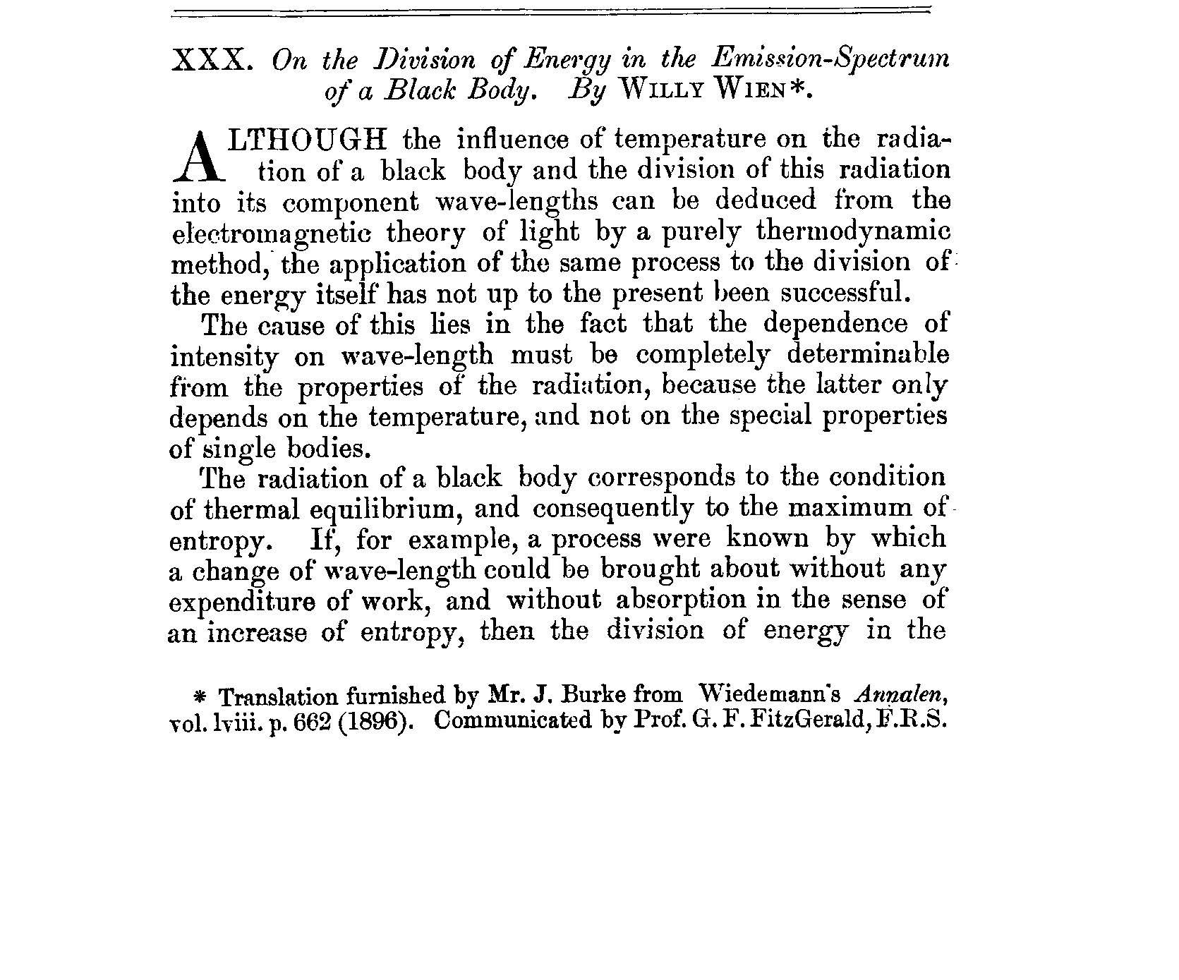
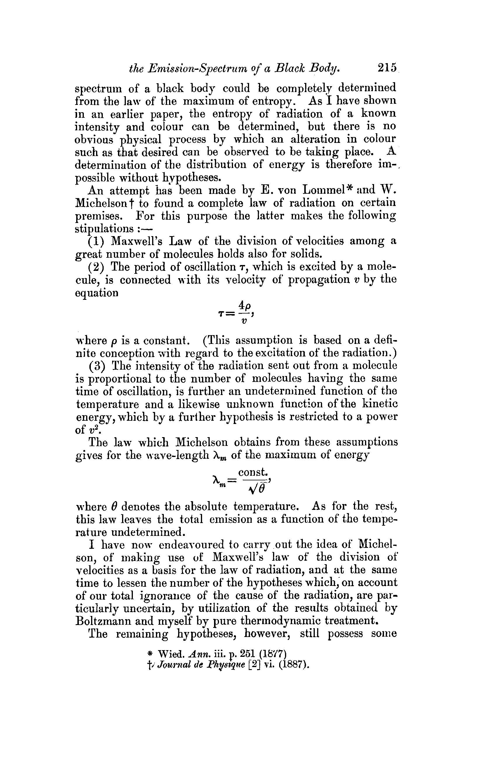

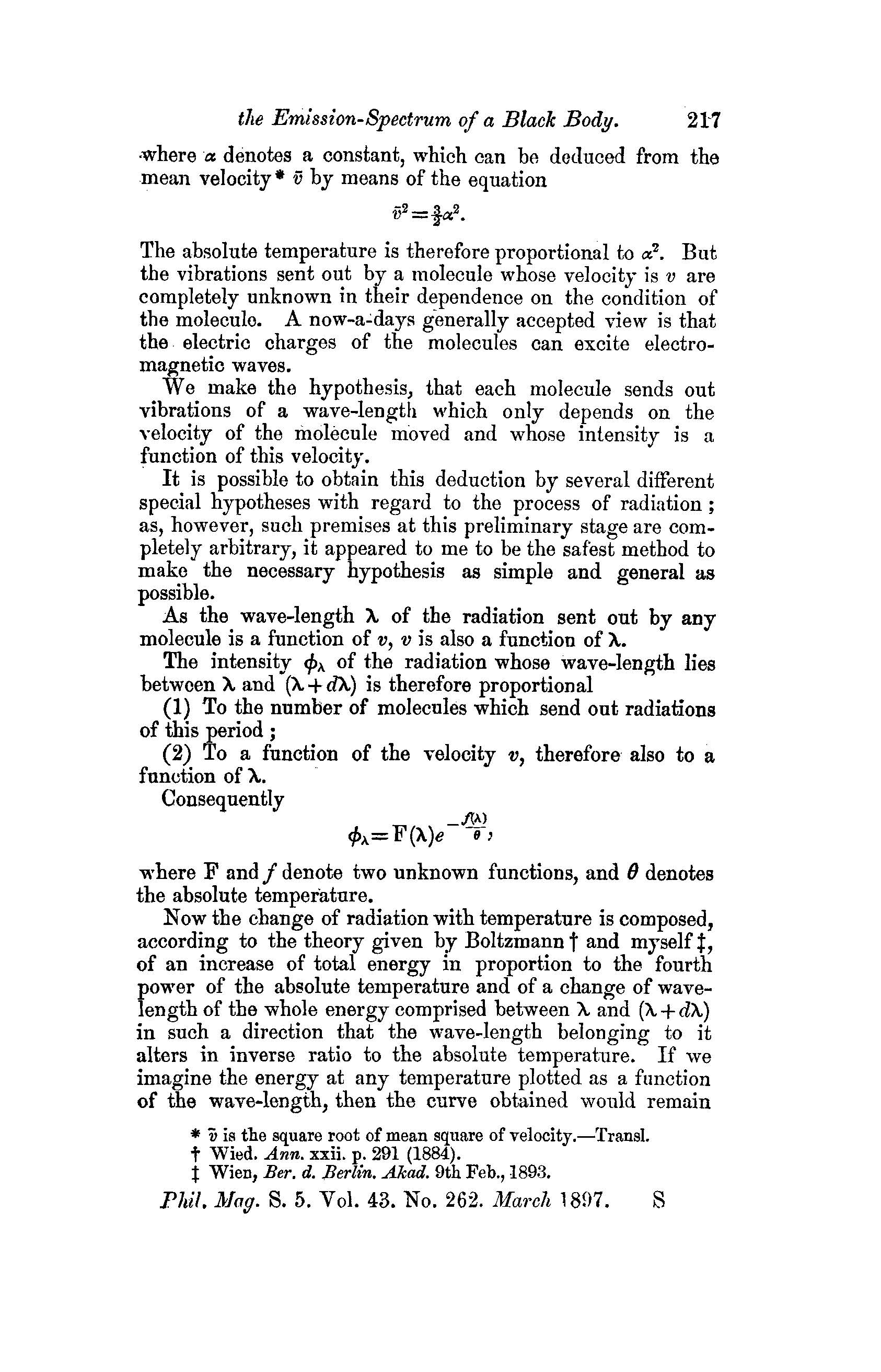
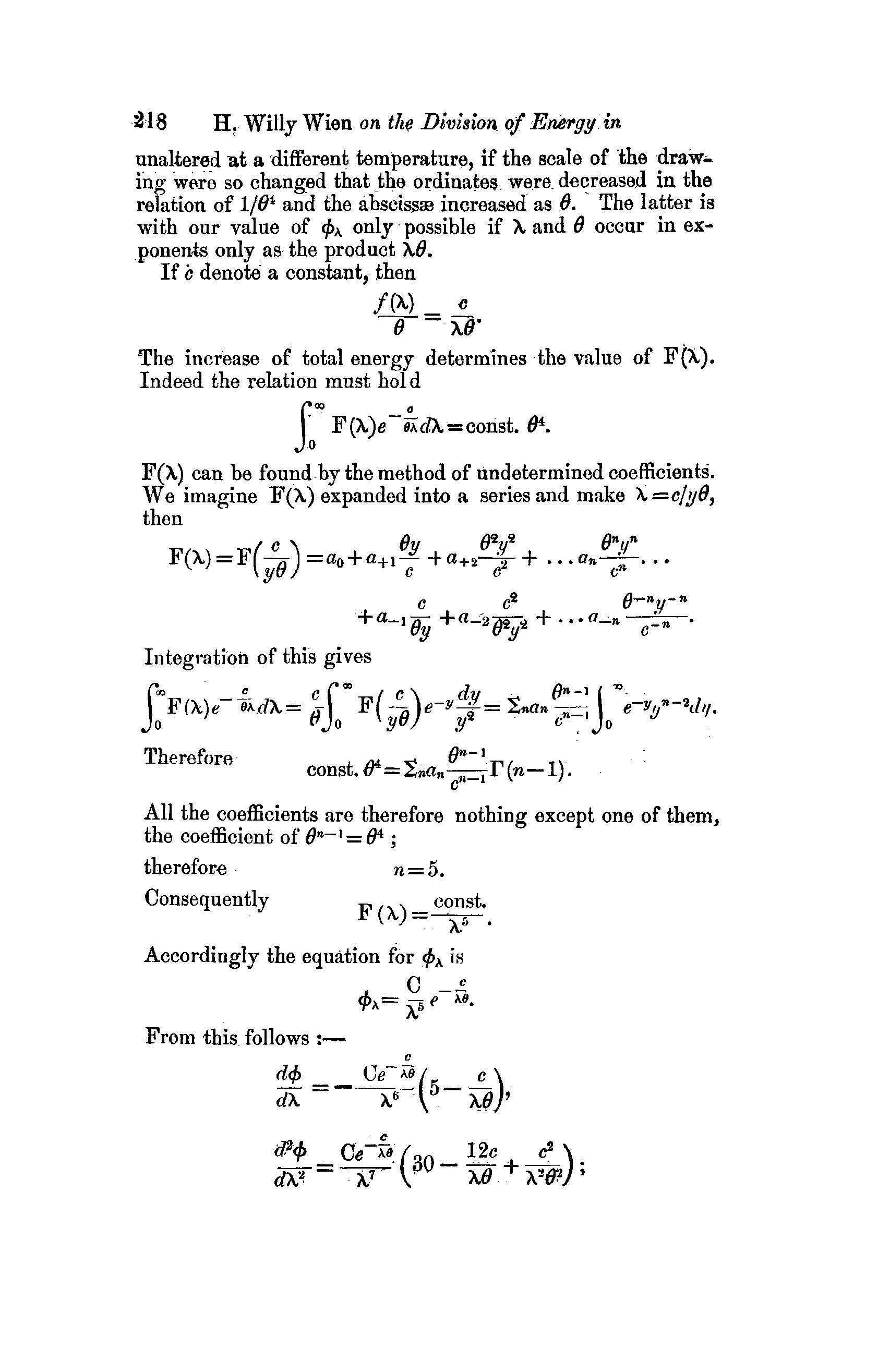
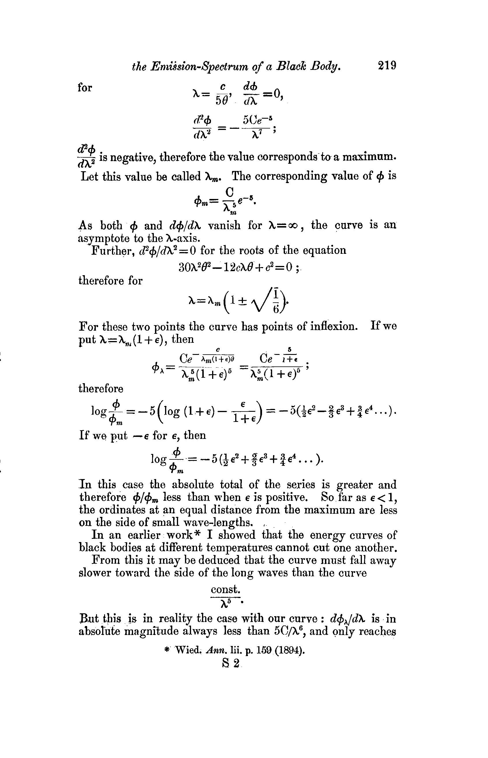
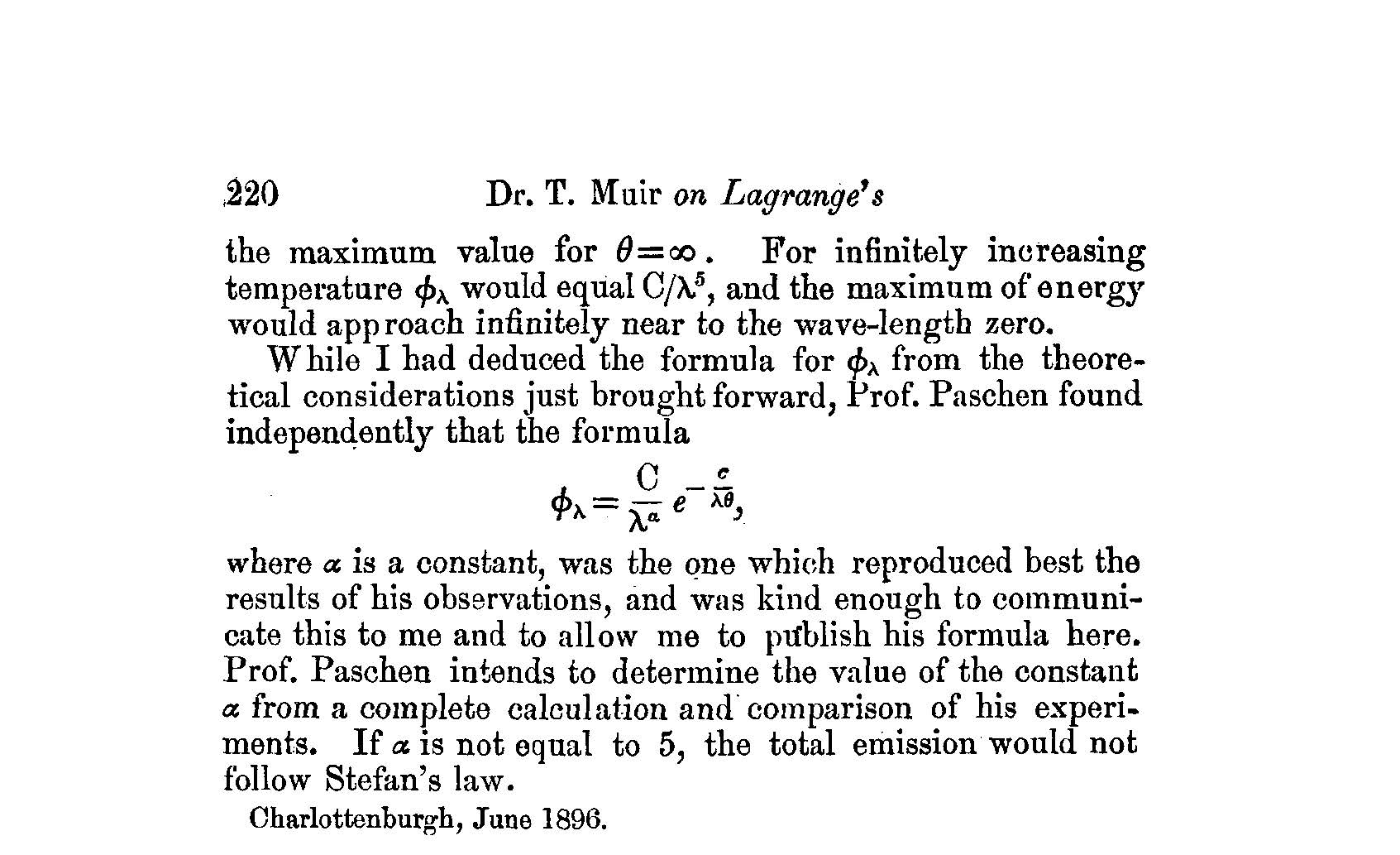
ADDENDUMEnglish Translation of Plancks Original 1901 Paper\(^{1}\)
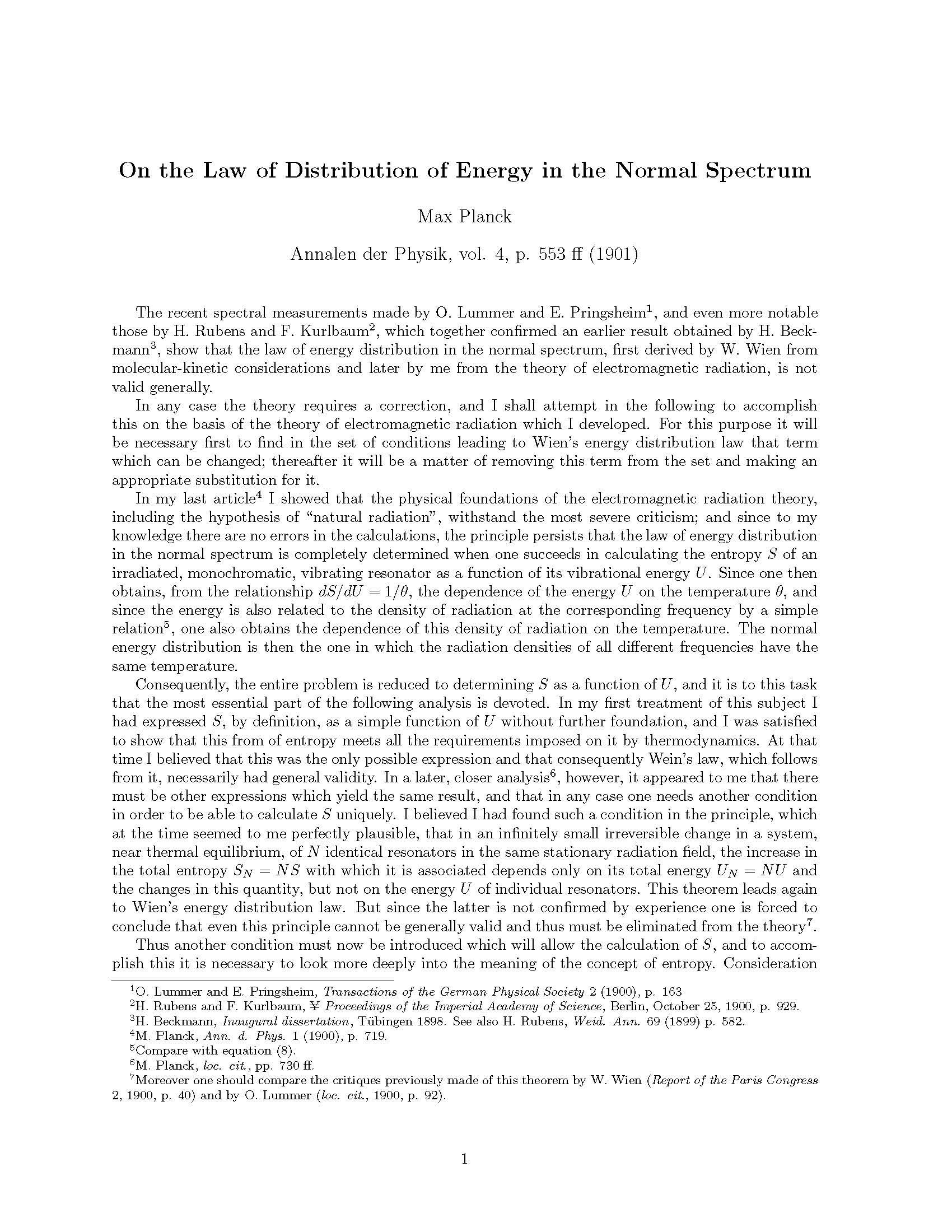
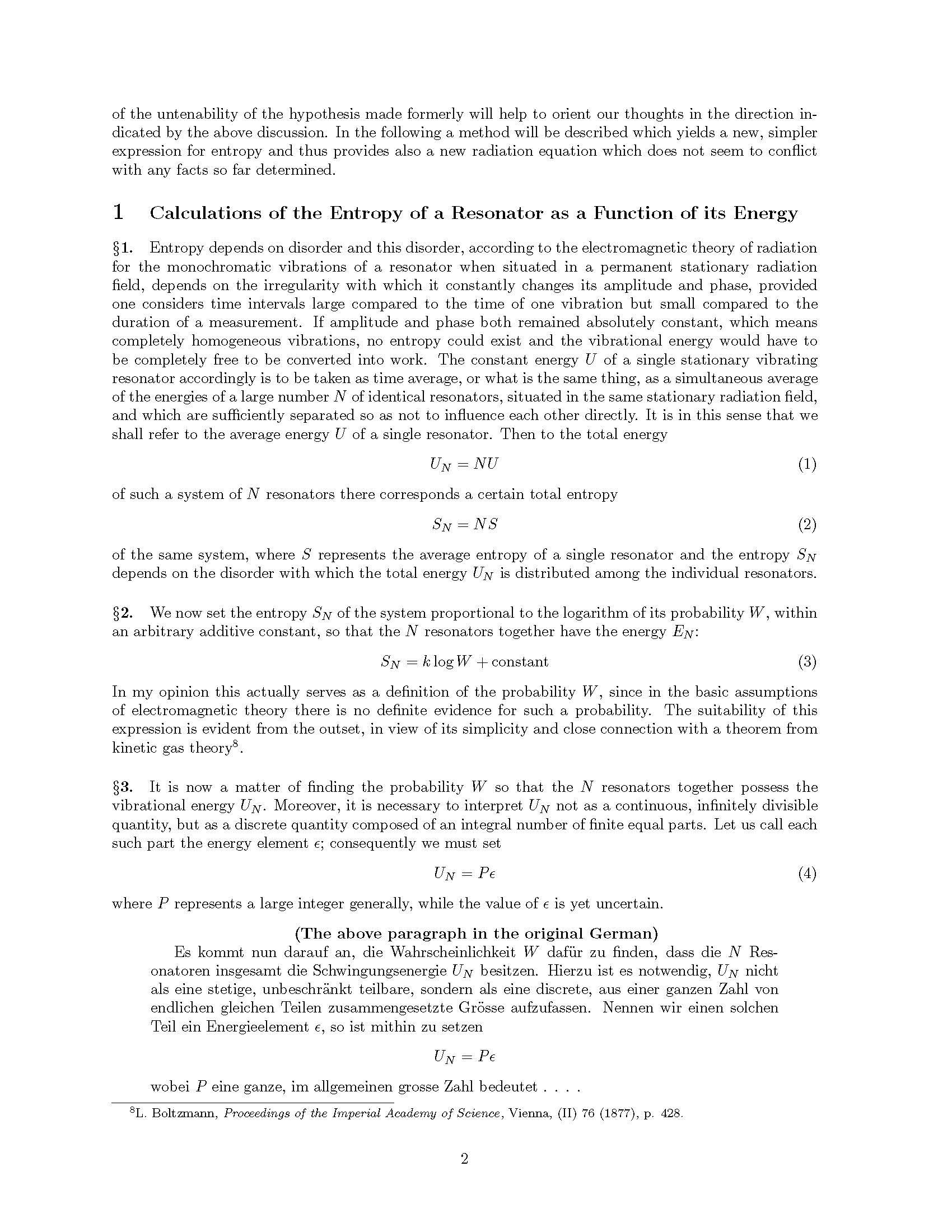

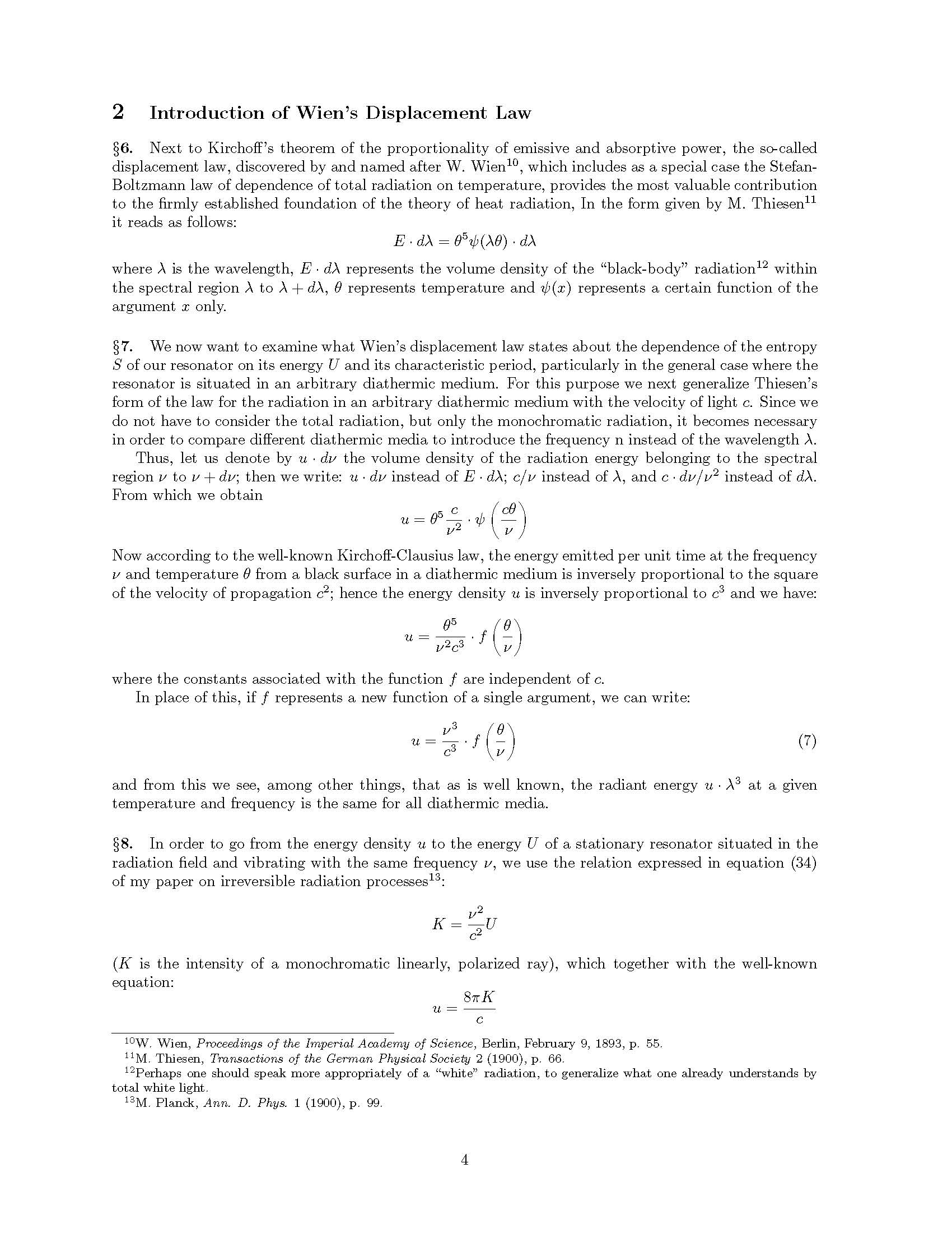
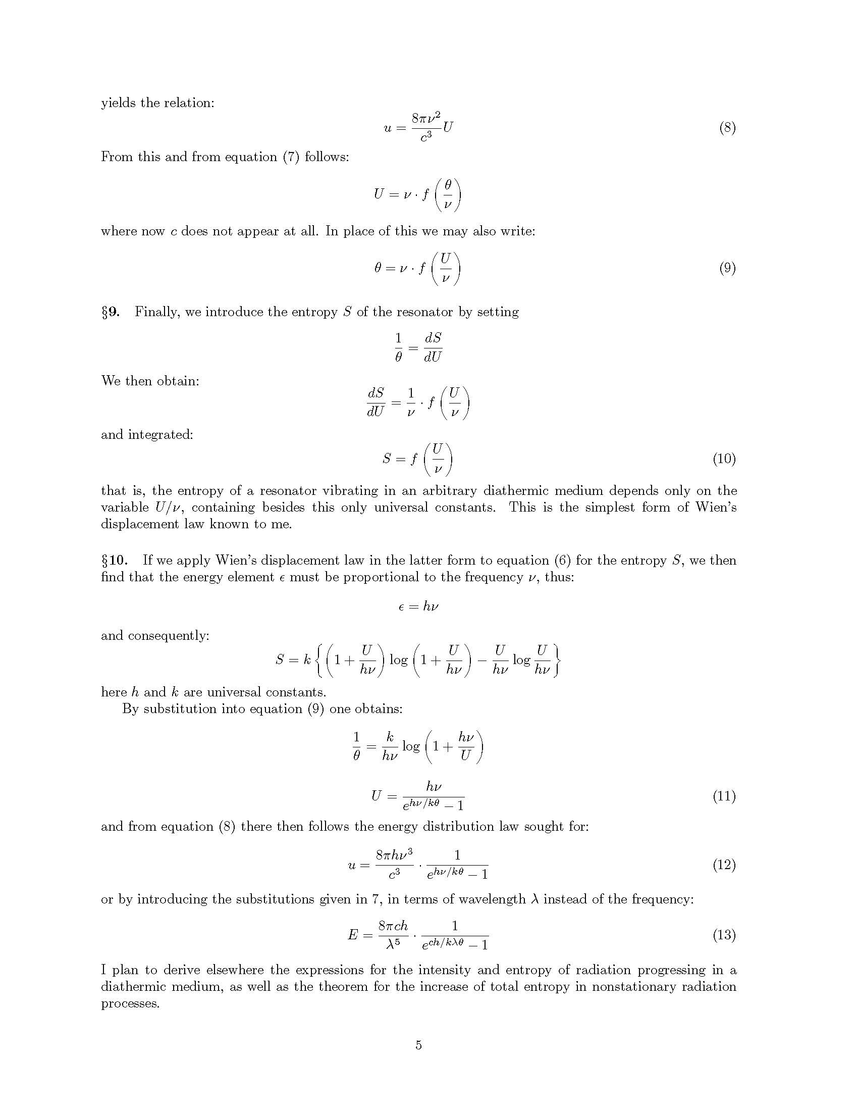
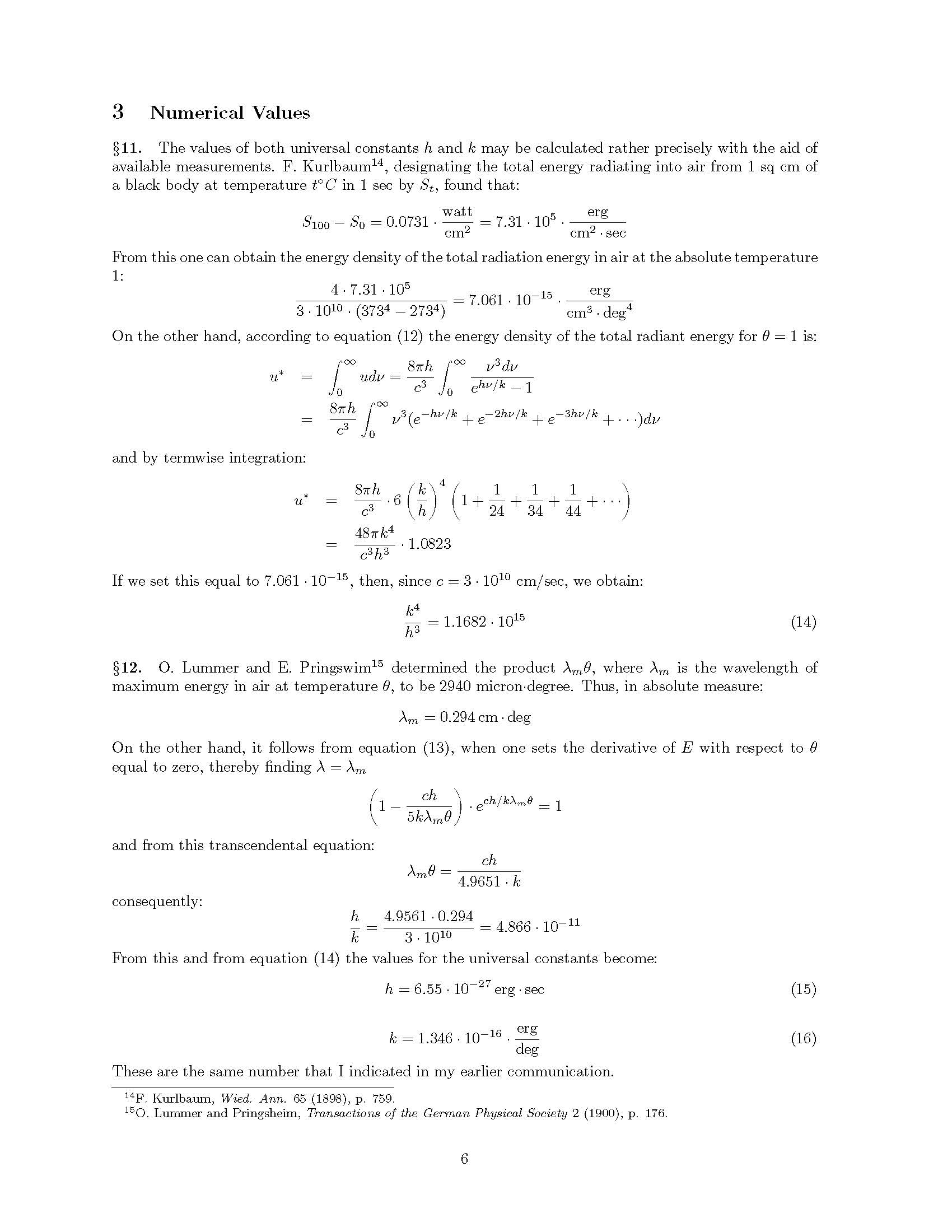
ADDENDUMC. I. Noninskis Paper\(^{11}\) (in Bulgarian)
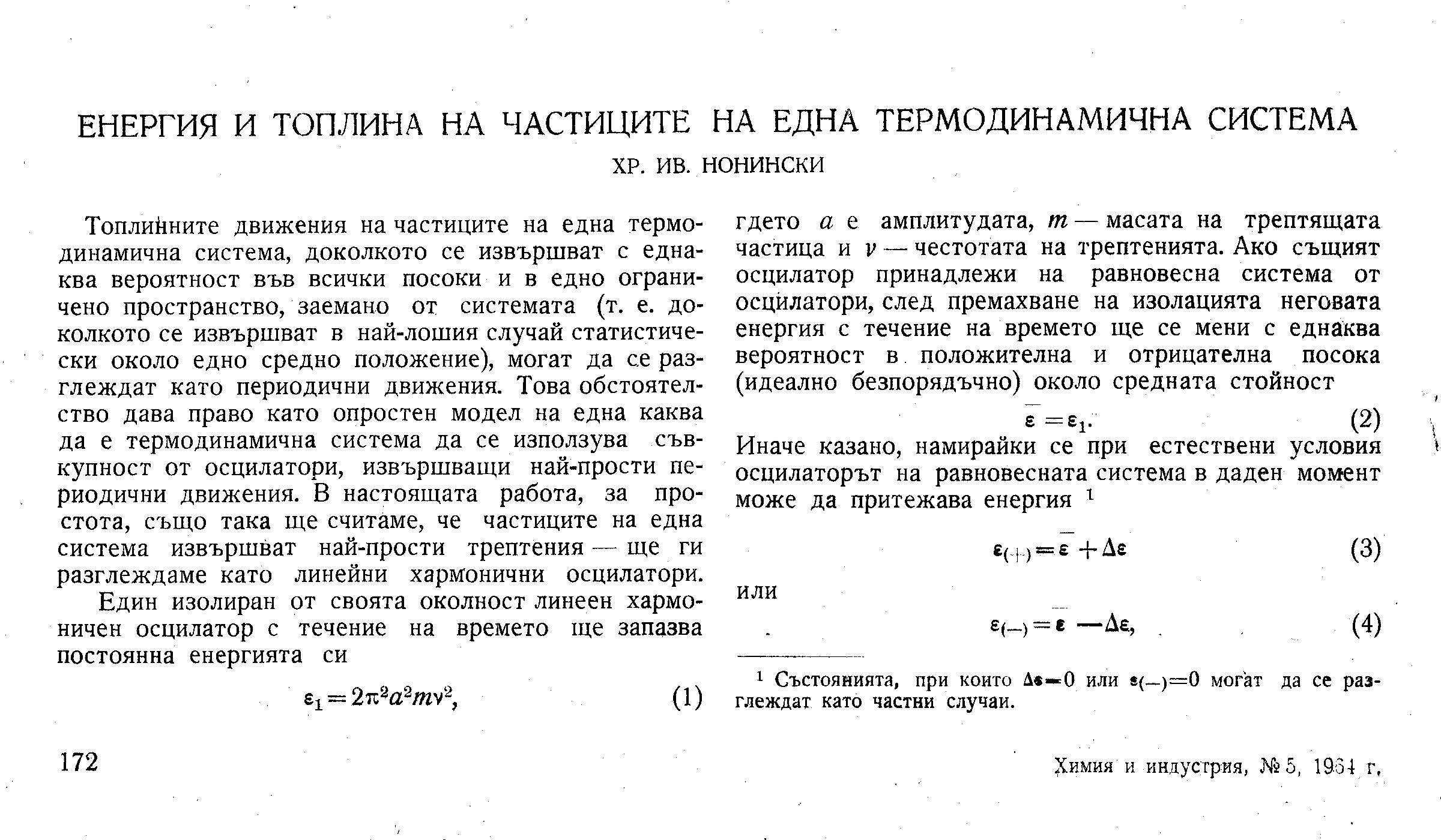

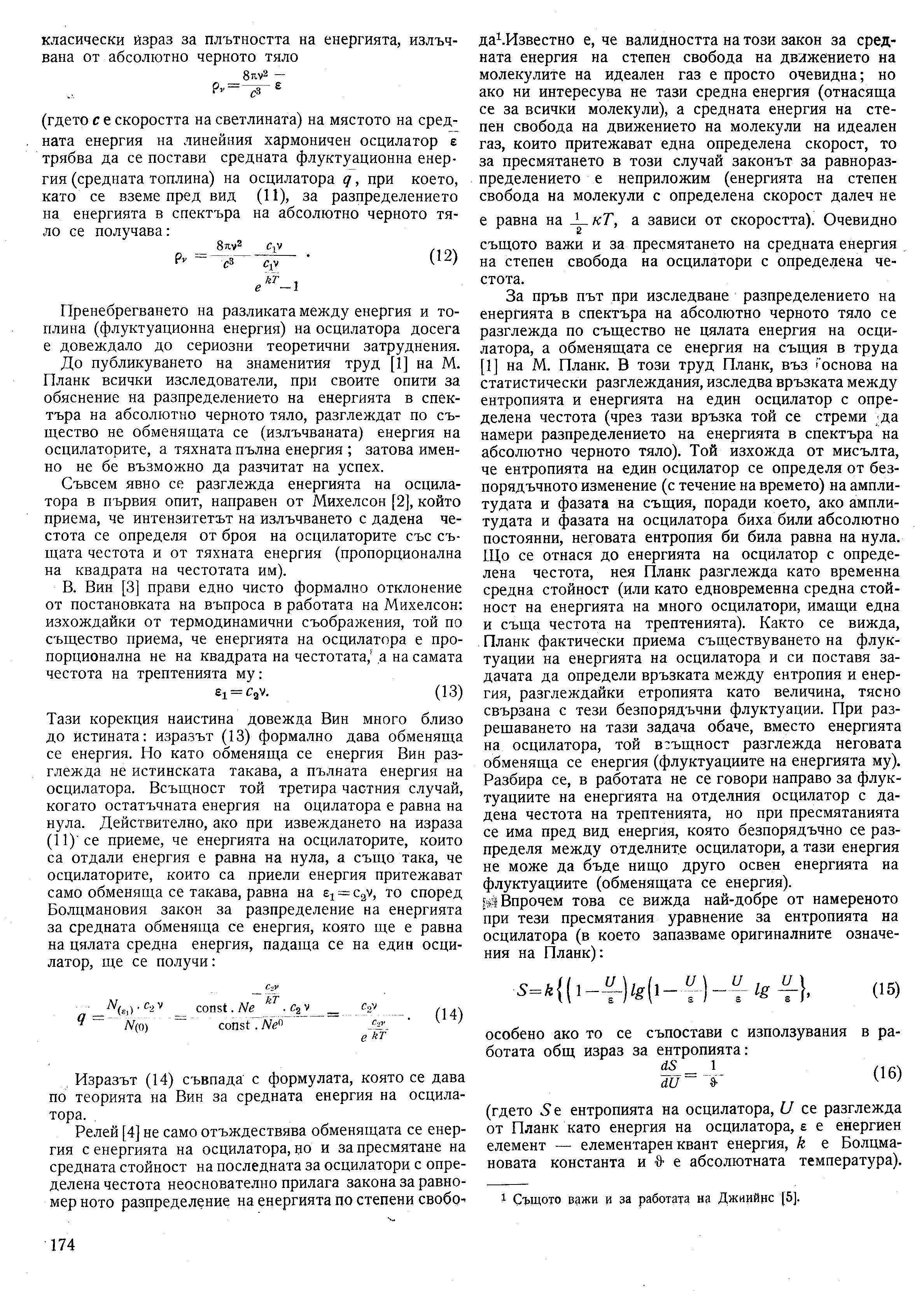
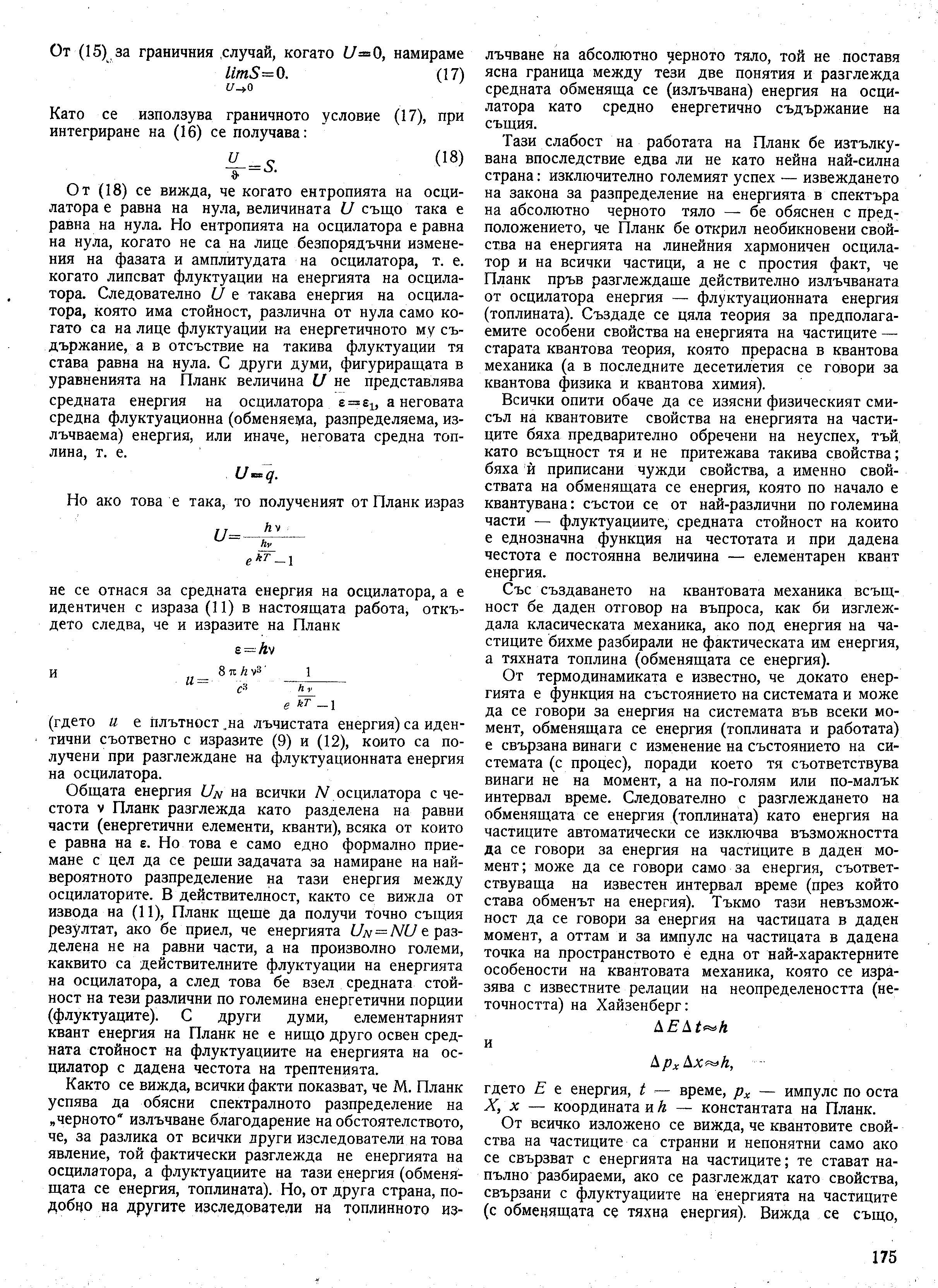
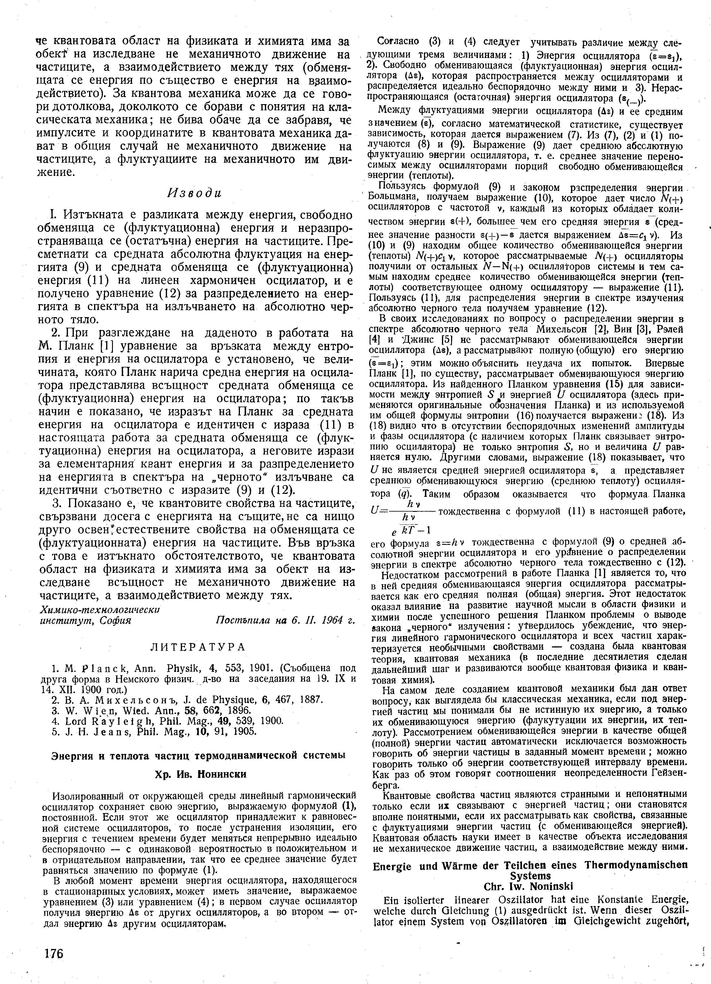

REFERENCES AND NOTES
1. Planck, M., Ueber das Gesetz der Energieverteilung im Normalspectrum, Ann. der Physik, 4, 553-566 (1901).
2. Einstein, A., Zur Qantentheorie der Strahlung, Phys.ZS., 18, 121-137 (1917).
3. Einstein, A., On the Electrodynamics of Moving Bodies in The Principle of Relativity, English translation of the original Einstein A., Zur Elektrodynamik bewegter Körper, Annalen der Physik, 17, 891-921, 1905, pp. 37-65 Dover, 1952.
4. Einstein, A., Über einen die Erzeugung und Vervandlung des Lichtes betreffenden heuristischen Gesichtspunkt, Annalen der Physik, 17, 132-148 (1905).
5. Einstein, A., On a Heuristic Point of View Concerning the Production and Transformation of Light, Annalen der Physik, 17, 132-148 (1905).
6. Einstein, A., Die Plancksche Theorie der Strahlung und die Theorie der spezifischen Wärme, Ann.Phys., 22, 180-190 (1907).
7. Einstein, A., Die Plancksche Theorie der Strahlung und die Theorie der spezifischen Wärme (Plancks Theory of Radiation and the Theory of Specific Heat), Annalen der Physik, 22, 180-190 (1907).
8. Noninski, V. C., Classical Bells Inequalities, Acta Scientiae,, 1, 91-92 (2008).
9. Noninski, V. C., A Qantum-Mechanical Measurement Leading to Simultaneous Spin-Up and Spin-Down of a Single Electron, Acta Scientiae, 1, 87-90 (2008).
10. Wien, W., , Wied.Ann., 58, 662 (1896).
11. Noninski, C. I., Energy and Heat of the Particles of a Thermodynamic System, Khimiya i Industriya (Sofia), 6, 172-177 (1964).
12. Noninski, V. C., Qantum Mechanics: Classical Mechanics of Exchange Energy (Heat) Rather Than Energy of the Particles Themselves, submitted, Phys.Rev.Lett., (2011).
13. Jordan, P., Über eine neue Begründung der Qantenmechanik. II., Z.Physik, 44, 1-25 (1927).
14. Carruthers, P. and Nieto, M. M., Phase and Angle Variables in Quantum Mechanics, Rev.Mod.Phys, 40, 411-440 (1968).
15. Davidson, E. R., On Derivations of the Uncertainty Principle, J.Chem.Phys., 42, 1461 (1965).
16. Yaris, R., Comment on On Derivations of the Uncertainty Principle, J.Chem.Phys., 44, 425-426 (1966).
17. Harris, R. A. and Strauss, H. L., Paradoxes from the Uncertainty Principle, J.Chem.Educ., 55, 374-375 (1978).
18. Michelson, A. A. and Morley, E. W., On the Relative Motion of the Earth And the Luminiferous Ether, Am. J. Sci., 34, 333-345 (1887).
19. Noninski, V. C., The Principle of Conservation of Energy Violated, Acta Scientiae, 1, 121-122 (2008).
20. Noninski, V. C., Everyday Violation of the Conservation of Energy Principle, Acta Scientiae, 1, 123-131 (2008).
21. Noninski, V. C., Crucial Conflict Between the Principle of Relativity (First Postulate of the Theory of Relativity) and the Lorentz Transformations, Acta Scientiae, 1, 13-17 (2008).
22. Noninski, V. C., Another Failed Attempt to Derive \(E = mc^2\) by Einsteins Theory of Relativity, Acta Scientiae, 1, 17-20 (2008).
23. Noninski, V. C., On the Invalidity of Einsteins Theory of RelativityIts Internal Contradictions, Which Exclude the Possibility of Experimental Validation, Acta Scientiae, Acta Scientiae, 1, 1-10 (2008).
24. Lummer, O. and Pringsheim, E., 1. Die Vertheilung der Energie im Spektrum des schwarzen Körpers und des blanken Platins; 2. Temperaturbestimmungfester glühender Körper, Verh. Deutsch. physik. Geselsch., 12, 215-235 (1899).
25. Noninski, V. C., On Einsteins Flawed Derivation of the Planck Radiation Law, Acta Scientiae,, 2, 119-120 (2011).
26. Noninski, V. C., Einsteins Theory of Relativity is Based on Internal Contradictions Which Make It Impossible to be Proved Experimentally, Acta Scientiae, 2, 121 (2010).
27. A, E., Does the Inertia of a Body Depend Upon Its Energy-Content? in The Principle of Relativity (English), pp. 67-71 Dover, 1952.
28. Nauenberg, M., Gap in Einsteins Early Argument for Existence of Photons Physics Today, 58, 17-18 (2005).
29. Cox, D. R. and Lewis, P., The Statistical Analysis of Series of Events Methuen, London, 1966.
30. Einstein, A., Podolsky, B. and Rosen, N., Can Quantum-Mechanical Description of Physical Reality Be Considered Complete?, Physical Review, 47, 777-780 (1935).
31. Bohm, D., A Suggested Interpretation of the Quantum Theory in Terms of Hidden Variables. I and II, Phys.Rev., 85, 166 and 180-193 (1952).
32. Bell, J. S., On the Einstein Podolsky Rosen Paradox, Physics, 1, 105-200 (1964).
33. Dirac, P. A. M., The Principles of Quantum Mechanics, 4th Ed. Oxford University Press, London, 1958.
34. Bohm, D., A Suggested Interpretation of the Quantum Theory in Terms of Hidden Variables. I, Phys.Rev., 85, 166 and 180 (1952).
35. Bohm, D., A Suggested Interpretation of the Quantum Theory in Terms of Hidden Variables. II, Phys.Rev., 85, 180-193 (1952).
36. Rayleigh, L., Remarks upon the Law of Complete Radiation, Phil.Mag., 49, 539-540 (1901).
37. Jeans, J., Phil.Mag., 10, 91 (1905).
38. Aerts, D., A mechanistic classical laboratory situation violating the Bell inequalities with 2.\( \sqrt{2}\), exactly in the same way as its violations by the EPR experiments, Helv.Phys.Acta, 64, 1-23 (1991).
39. Bell, J. S., Foundations of Qantum Mechanics, Ed. B. Espagnat, Academic Press, New York, 1971.
40. Couder, Y. and Fort, E., Single-Particle Diffraction and Interference at a Macroscopic Scale, Phys.Rev.Lett.,, 97, 154101-1,4 (2006).
41. Noninski, V. C., Qasi-Equilirium Clustering Upon Supersaturation in Homogeneous Phase Formation, J. Crystal Growth, 97, 497-501 (1989).
42. Noninski, V. C., Stable Drop at Positive Line Tension, Colloids Surfaces, 42, 205-207 (1989).
43. Noninski, V. C., Small Stable Drops and Crystals in Supersaturated Homogeneous and Heterogeneous Systems at Positive Specific Linear Free Energy, J. Colloid Interface Sci., 143, 374-381 (1991).
44. Binnig, G. and Rohrer, H., Scanning Tunneling Microscope, Helv. Phys. Acta, 55, 726-735 (1982).
45. Binnig, G., Rohrer, H., Gerber, C. and Weiber, E., 7 x 7 Reconstruction of Si(111) Resolved in Real Space, Phys. Rev. Lett., 50, 120-123 (1983).
46. Noninski, C. I., On the Thermodynamic Stability of the Disperse Buildup of the Crystals, Khimia i Industriya (Sofia), No.5, 33, 144-151 (1961).
47. Noninski, C. I., On Some Consequences from the Equation Connecting the Surface Tension of a Spherical Drop (Small Crystal) With Its Radius, Khimia i Industriya (Sofia), 39, 208-211 (1967).
48. Kroto, H. W., Heath, J. R., OBrien, S. C., Curl, R. F. and E., S. R., C60: Buckminsterfullerene, Nature, 318, 318 (1985).
49. Handbook of Chemistry and Physics, 73rd Edition, David, R. Lide, Editor-in-Chief, CRC Press, Boca Raton, Fl, 1992-1993.
50. Noninski, C. I., On the Wave Properties of the Electron, Annual of the State Polytechnic, 4, 141-163 (1953).
51. Noninski, C. I., Private communication. C. I. Noninski vehemently opposed any sug-gestion that conservation of energy (CoE) can be violated. This author challenges such impossibility in a forthcoming book.
52. http://hypertextbook.com/facts/2000/ DannyDonohue.shtml,.
53. Pauling, L., College Chemistry, pp. 57, 45 Freeman, San Francisco, 1964.
54. http://www.newton.dep.anl.gov/ newton/askasci/1993/physics/PHY112.HTM,.
55. Sokal, A. and J., B., Fashionable Nonsense, Editions Odile Jacob, 1999.
56. Popper, K. R., Conjectures and Refutations: The Growth of Scientific Knowledge, pp. 33-39 BASIC BOOKS, Publishers, New York, London1962.
57. Tribe, L. H., The Curvature of Constitutional Space: What Lawyers Can Learn From Modern Physics, Harv. L. Rev., 103, 1-40 (1989).
58. Einstein, A., Über die von der molekularkinetischen Theorie der Wärme geforderte Bewegung von in ruhenden Flüssigkeiten suspendierten Teilchen Annalen der Physik, 17, 549-560 (1905).
59. Noninski, V. C. and Noninski, C. I., Physical Molecule. 60-Molecular Thermodynamically Stable ParticleThe Building Entity of Liquids and Solids, Acta Scientiae, 1 (2008).
60. Discussion of the conservation and the transformation aspect of CoE will be done elsewhere.
61. Neither distance, nor force are energy, nor are they nothingtheir product is work (spent energy); the same applies to current and voltageneither current, nor voltage are energy (or energy per unit time; i.e., power), nor are they nothingtheir product, however, is power.
62.This should come as no surprise because we already know that not just any \(\nu\) will result in a standing wave and \(\lambda\) is connected with \(\nu\) via \(\lambda \nu = c\).
63.Alternatively, this absolute fact is expressed by time-dilation is absolutely impossible and no experiment is expected to prove otherwise. This also means that there is no such thing as simultaneity is relative is non sequitur. On the contrarysimultaneity is absolute. The absolute impossibility to ever expect time-dilation stems from the absolute truth that spatially coinciding clocks are synchronous; that is, that time at a given moment, in a given place, cannot have two different values. Regarding absoluteness of simultaneity consider the following: It is an absolute truth that spatially coinciding clocks are always synchronous. If clocks, moving or not, at any instant of time spatially coincide in the stationary system, then their own coordinate systems also coincide and, therefore, they are synchronous also in their own systems. Now, because all stationary clocks are synchronous, according to the simple synchronization procedure, and because the, say, a moving clock inevitably coincides with one of these resting synchronous clocks at any moment of time, the following is clear: From the absolute truth that all spatially coinciding clocks are synchronous, it follows that the the moving clock is synchronous with all synchronous stationary clocks at any given moment. Therefore, it is an absolute truth that the rate of time measured by the a moving clock is the same as the rate of time measured by the stationary clocks. Therefore, not only are Lorentz transformations corrections not needed for the moving clocks but also, more importantly, time dilation is an absolute impossibility. The only corrections of time that need to be made on a moving clock are corrections due to the finite speed of signals, but this is a trivial matter, having nothing to do with relativity.
64. This alternatively is expressed as length-contraction is absolutely impossible. The arguments for this absolute fact also stem from the argument given in the previous footnote, basically based on the absolute fact that two spatially coinciding clocks are synchronous.
65. Probably, for a better understanding of the above internal contradiction, it would help to demonstrate the flaw in that erroneous derivation algebraically. What is claimed in ref.\(^{2}\) is akin to claiming that because \begin{equation}\label{eq3_|_} b_1 = const . f_1(x) \left( b_2 + \frac{a} {f_2(x)} \right) \end{equation} becomes \begin{equation}\label{eq4_|_} b_1 = const . b_2 \end{equation} due to the fact that \(f_1(x) \rightarrow 1\) and \(f_2(x) \rightarrow \infty\) when \(x \rightarrow \infty\), we are allowed to write \begin{equation}\label{eq5_|_} const . b_2 = const . f_1(x) \left( b_2 + \frac{a} {f_2(x)} \right). \end{equation}
The substitution of eq.(\ref{eq4_|_}) into eq.(\ref{eq3_|_}) to obtain eq.(\ref{eq5_|_}), however, is obviously illegitimate since eq.(\ref{eq3_|_}) is a function of \(x\) while eq.(\ref{eq4_|_}) is not. Furthermore, eq.(\ref{eq4_|_}) is not an absolute equality but is constrained by the condition \(x \rightarrow \infty\) and cannot be used without that constraint. Thus, for values of \(x\) where eq.(\ref{eq3_|_}) is valid eq.(\ref{eq4_|_}) is invalid. The seeming similarity of the substitution the author of ref.\(^{2}\) did with the boundary value problems in differential equations is misleading, because in the boundary value problems, the equalities expressing the boundary conditions themselves are absolute; that is, these equalities themselves are unrestrained by constraints. On the other hand, the solution of a differential equation with boundary conditions (constraints) is a function which is not a generalized result but obeys the original conditions under the given constraints only. As an example \(y(x) = 2 sin(x)\) is not the general result as a solution of the differential equation \(y''(x) + y(x) = 0\) but is a special one satisfying \(y(0) = 0\) and \(y \left(\frac{\pi}{2}\right) = 2\).
66. Thus, by varying we mean just a change by a small portion of a given quantity, not treating that quantity as a function of something else, in which case we would take, instead, the differential of that function of that something else. By varying something, signifying that varying by writing in front of it the symbol \(\delta\), we mean specifying of a small chunk, a crumb or a morsel of it (if there is a difference between a crumb and a morsel), treating that something as a given whole entity. Thus, one may imagine, in case of a function, that \(\delta y\) is only the main part of the change of the function \(y = y(x)\) (that is, the part participating as a denominator in the derivative \(\frac{dy}{dx}\) of the function), while \(\delta y\) is the entire infinitesimal change of the function \(y = y(x)\).
67. Trying to fit too much information and explanation about a notion, aiming at making the text shorter, may be confusing, but at least it's there. Here, outside of the main text, there is even more explanation: The first law of thermodynamics is a simple accounting regarding what contributes to positive change of the internal energy \(U\) of the system. Thus, the law concerns just the change, the contribution, how much and what is added to the system to increase \(U\), not the internal energy \(U\) itself, which the system contains. The first law identifies the two ways of increasing \(U\)through transfer of portion \(\delta q\) of heat and through doing work \(\delta w_{volume \ work}\) on the system. Now, while expressing the portion of heat is at once comprehensible, once we've been exposed to the notion of entropy \(S\rightarrow dS=\frac{\delta q}{T}\), hence, \(\delta q = TdS\), expressing the work \(\delta w_{volume \ work}\) done on the system may cause slight confusion with regard to its sign. To make it clear, imagine the observed system inside a cylinder with a piston. When work is done on the system the piston squeezes the inside, reducing the volume. When reduction of volume takes place, it can be expressed by subtracting a larger, initial, value from a smaller, reduced, value. Therefore, the change \(dV\) itself will have a negative sign, despite the fact that work is done on the system and the system gains energy. Thus, the work \(PdV\), which has been expended by the surroundings, would appear negative from the point of view of the system if we dont do something (if we dont change the sign). Thus, by changing the sign, this \(PdV\) becomes a positive contribution, a positive quantity, from the point of view of the system, as far as the internal energy \(u\) of the system goes. Therefore, \(dU = TdS - PdV\), where the minus sign compensates the negative value \(PdV\), making that value a contributor, alongside \(TdS\), to the gain in internal energy \(dU\). The minus sign may be easier to understand, if the system is doing work on the surroundings, which means the system is losing energy. But, then, the system will be expanding and the \(dV\) as well as \(PdV\) will be positive. However, in this case, when the system expands, that quantity \(PdV\) is internal energy (expressed as work) which the system loses. Therefore, \(PdV\) must be subtracted when it comes to the contribution \(dU\) to the energy of the system and, as a result, the two contributions to the increase of the energy of the system \(dU\) are \(dU = TdS - PdV\).
68. Here and here a special point was made that the ideal (universal) gas law must not be used when deriving a relation between macro-quantities, such as the quantities participating in the ideal gas law, from the micro-quantities of the molecular-kinetic theory. In contrast, in the current case, the derivation is entirely within the macro-frame of thermodynamics. Therefore, substitution of the ideal gas law is fully justified.
69. Before going into the exact details of the concrete botched derivation in ref.\(^{4}\), with the actual quantities in the equations, we will resort to a simple example, in order to understand clearly the flaw. Thus, imagine it is given that \(\ln \frac{y}{x^3} = const\), where \(y = y(x)\). Then, the question follows: What is \(\int \ln \frac{y}{x^3} dy\) equal to? The answer to this question must necessarily be \(\int \boxed{\ln \frac{y}{x^3}} dy = \boxed{\ln \frac{y}{x^3}} \int dy = y \ln \frac{y}{x^3} + C\). However, instead of appreciating that it is the entire expression \(\ln \frac{y}{x^3}\) that is a constant in its togetherness, and therefore \(\ln \frac{y}{x^3}\) is not a function of \(y\), neither is it a function of anything else, allowing to be factored out of the integral, the author\(^{4}\) decides, contrary to logic, to observe that expression \(\ln \frac{y}{x^3}\) as a function of one of its component quantities, \(y\), writing \(\int \ln \frac{y}{x^3} dy = y \left( \ln \frac{y}{x^3} - 1 \right) + C \).
70. Now, let us see how it translates in the real terms of the paper. Thus, eq.(\ref{dphi}), \(d \varphi = -\frac{1}{\beta \nu}\ln \frac{\rho}{\alpha \nu^3} d \rho = const . \rho\), the last, rearranged, equation before integration can now be integrated correctly, honoring the inescapable fact that the entire expression \(-\frac{1}{\beta \nu}\ln \frac{\rho}{\alpha \nu^3}\) in its togetherness is a constant. It is not a function of \(y\), despite the visible presence of \(y\) in it. Therefore, it can be at once factored out of the integral (as a reminder, we present symbolically, albeit redundantly, after the second equality, what happens with the \(const\) in the course of integration) \begin{equation*} \int d \varphi = \int \underbrace{-\frac{1}{\beta \nu}\ln \frac{\rho}{\alpha \nu^3} }_\text{const} d \rho = \int const \cdot d\rho \end{equation*} \begin{equation*} \int d \varphi = \underbrace{-\frac{1}{\beta \nu}\ln \frac{\rho}{\alpha \nu^3} }_\text{const} \int d \rho = const \int d\rho \end{equation*}
yielding \begin{equation}\label{correctphi} \varphi = -\frac{\rho}{\beta \nu}\ln \frac{\rho}{\alpha \nu^3} = const \cdot \rho, \end{equation}
which, then, can have both sides of the equality, as well as the numerator and the denominator of the quotient after the logarithm, multiplied by \(v\), giving, for a given \(\nu\) \begin{equation}\label{entropyfromphi} v \varphi = S = -\frac{v\rho}{\beta \nu}\ln \frac{\rho}{\alpha \nu^3}. \end{equation}
Of course, we can also have the numerator and the denominator of the quotient after the logarithm, multiplied by \(v\), as the author has done, \(v \varphi = S = -\frac{v\rho}{\beta \nu}\ln \frac{v\rho}{v\alpha \nu^3} = -\frac{E}{\beta \nu}\ln \frac{E}{v\alpha \nu^3}\), with the goal to get the energy of radiation \(E\) into the equation. He desperately needs that multiplication, in order to somehow get the logarithm of the quotient of the two volumes when expressing \(S - S_0\), thus, proving the analogy with the thermodynamic (implying discreteness) formula \(S - S_0 = \frac{E}{\beta \nu}\ln \frac{v}{v_0}\). However, we see at once the uselessness of that multiplication by \(v\) of the quotient after the logarithm, considering that \(v\rho = E \ne v_0 \rho = E_0\).
Therefore, even if we accept that the frequency \(\nu\) stays the same when the volume changes from \(v\) to \(v_0\), even then we cannot ignore the absolute fact that \(v\rho = E \ne v_0 \rho = E_0\) when trying to form the sought for difference \(S - S_0\) when changing the volume of the blackbody enclosure from \(v\) to \(v_0\), using eq.(\ref{entropyfromphi}) \begin{equation*} S - S_0 = -\frac{v\rho}{\beta \nu}\ln \frac{\rho}{\alpha \nu^3} + \frac{v_0\rho}{\beta \nu}\ln \frac{\rho}{\alpha \nu^3} \end{equation*}
or \begin{equation}\label{sminuss0fromWien} S - S_0 = (v_0 - v) \frac{\rho}{\beta \nu}\ln \frac{\rho}{\alpha \nu^3}. \end{equation}
The above expression, eq.(\ref{sminuss0fromWien}), for the \(S - S_0\) difference, obtained from Wiens law, resembles the expression \(S - S_0 = (v - v_0)\frac{\rho}{\beta \nu} \ln \left( \frac{\alpha \nu^2}{\rho} + 1 \right)\), for this ostensible entropy difference, obtained from Plancks law, both of these expressions having nothing to do with the thermodynamic relation \(S - S_0 = \frac{E}{\beta \nu} ln \frac{v}{v_0} = R ln \frac{v}{v_0}\).
71. The first part of ref.\(^{6}\) is rejected due to inadequacy of the probability \(dW = C e^{- \frac{E}{kT}} dx_1, dx_2 \dots dx_m\) formula. We do not need to invoke probability regarding whether the coordinates \(x_1 \dots x_m\) belong to the region \(dx_1, dx_2 \dots dx_m\), for it is exactly these parameters \(x_1 \dots x_m\) that determine the region and its energy \(E\). Thus, the Boltzmann factor \(e^{- \frac{E}{kT}}\) is redundant since the probability that \(x_1 \dots x_m\) belong to the region \(dx_1, dx_2 \dots dx_m\) is one hundred per cent.
72. Indeed, the quotient itself \(\frac{0 + A \varepsilon e^{-\frac{N}{RT}\varepsilon} + A 2\varepsilon e^{-\frac{N}{RT}2\varepsilon} ...}{A + A e^{-\frac{N}{RT}\varepsilon} + A e^{-\frac{N}{RT}2\varepsilon} + ...} = \frac{ \varepsilon \left( e^{-\frac{N}{RT}\varepsilon} + 2 e^{-\frac{N}{RT}2\varepsilon} ... \right) }{1 + e^{-\frac{N}{RT}\varepsilon} + e^{-\frac{N}{RT}2\varepsilon} + ...}\), taken as just a mathematical expression, resembles the quotient of the infinite sums \(\frac{x \sum\limits_{n = 1}^{n = \infty} {ne^{-n x}}}{\sum\limits_{n = 0}^{n = \infty} {e^{-n x}}} = \frac{x\frac{e^x}{(e^x - 1)^2}}{\frac{e^x}{e^x - 1}} = \frac{x}{e^x - 1}\), which, after substitution of \(x\) by \(\varepsilon\) and the coefficient \(\frac{N}{RT}\) before \(\varepsilon\), becomes \(\frac{\varepsilon}{e^{\frac{N}{RT}\varepsilon} - 1}\).
73. Rayleighs formula is deficient and had to be replaced by Plancks formula, because Rayleigh considered that the density of modes \(\frac{8\pi \nu^2}{c^3}\) must multiply the same average energy \(kT\) at every frequency because of the equipartition theorem (a resonator has \(2\) degrees of freedom, which, multiplied by \(\frac{1}{2}kT\) per degree of freedom makes \(2 \times \frac{1}{2}kT = kT\)). However, that \(kT\) is average energy of a particle when considering the entire ensemble, while the energy of the individual members of that ensemble is varying, spread according to a distributiona Gaussian or, more precisely, Poissonand therefore, rather than \(kT\), the mean energy which must be multiplied by the density of modes must have the form \(\frac{h\nu}{e^{\frac{h\nu}{k\theta}}-1}\), which, as seen later is, in fact, \(\overline{q} = \frac{\mathscr{h}\nu}{e^{\frac{\mathscr{h}\nu}{kT}}-1}\).
74. More exactly, for the mean value of the portions of exchange energy transferred amongst the resonators (mean absolute value of the energy fluctuations of the resonator) we get \begin{equation}\label{MeanFluctuation} \scriptsize \overline{ \left| \Delta \varepsilon \right| } = \sqrt{\frac{2} {\pi} } \sqrt{ \overline{ \left( \Delta \varepsilon \right)^2 } } = \left( \sqrt{\frac{2} {\pi} } \sqrt{ \varepsilon_0 2 \pi^2 A^2 m } \right) \nu = \mathscr{h} \nu, \end{equation} where the expression in the parentheses after the second equality, is a constant, which we denote by \(\mathscr{h}\), to distinguish its arrival in C. I. Noninskis derivation from the seeming arrival, in fact, as a result of curve-fitting adjustment, rather than from derivation, of constant \(h\) in Plancks paper\(^{1}\), a constant having a numerical value evaluated in the same way, using the same experimental data provided by experiments such as those of Lummer and Pringsheim\(^{24}\), which led Planck to calculate the value of his constant \(h\) in part \(3\) \(\S11\) and \(\S12\)) of his paper\(^{1}\).
75. Although we need not involve ourselves with more mathematical detail than the minimum detail needed to reveal the mathematical problems of quantum mechanics, occasionally, it may be appropriate to give a brief clarification of terms used. Thus, eigenfunction equation is such an equation, whereby an operator (hold on, what is an operator will be defined in a minute) applied to a so-called eigenfunction, in this context a state function or a state vector, which is a specific function associated with the operator, a function possessing this particular property to result in being scaled; that is, resulting in that same function being multiplied by a constant. Here is the promised explanation of what an operator isfor the purposes of our discussion, an operator is a certain mathematical construct, say, a matrix, which is pronounced to represent an observable, such as, for example, position, momentum or energy. When the operator is applied to the eigenfunction associated with that operator, the operator extracts form that eigenfunction the scaling factor called eigenvalue. This seems just about the simplest explanation of an eigenfunction equation, with the addition that the eigenfunction can alternatively be represented as an eigenvector. Incidentally, we need not worry how operators come about. The only thing of interest is how these operators, which are already presented to us, behave in the discussed context, and whether or not the outcomes have a physical meaning (as a heads-up, they dont, and this is exactly what we are about to have demonstrated).
76. Hilbert space is a vector space; that is, a vector manifold, which is characterized by a particular (may be even infinite) set of unit vectorsthe so-called basis of the vector spacewhich may generate every possible vector belonging to that space by their linear combination. Also, a given vector space is defined by rules which govern that space. For instance, the basis of the Hilbert space is orthonormal; that is, each one of the vectors comprising the basis, is a unit vector, and all of these unit vectors comprising the basis, are perpendicular to each other. Also, the Hilbert space is governedby a particular way the vectors form inner (scalar) products. What is especially important for us is that the inner product of a vector with its own complex conjugate in the Hilbert space must be finite (must be unity if that inner product is of a vector of the basis). The result \(0\) or \(\infty\) of a claimed vector inner product indicates that the vector in question does not belong to the Hilbert space; that is, such vector is non-physical. It is assumed that only vectors which belong to the Hilbert space have physical meaning (heads-upall eigenvectors we will encounter below, are non-physical, because their normalization does not result in a finite non-zero number, ergo they dont belong to the Hilbert space).
77. In momentum space the position operator \(\widehat{x}\) is \(i \hbar \frac{d}{dp}\) and the momentum operator \(\widehat{p}\) is \(p\).
78. The delta-function \(\delta(a - a)\), according to the Cauchy definition is \begin{equation*} \delta(a - a) = \frac{1}{2 \pi}\int\limits_{-\infty}^{+\infty} e^{i y (a - a)} dy, \end{equation*} and, because \((a - a) = 0\), the value of the exponent \(e^{i y (a - a)}\) is unity, and therefore we end up with the integral \begin{equation*} \delta(a - a) = \frac{1}{2 \pi}\int\limits_{-\infty}^{+\infty} dy = \infty, \end{equation*} which does not converge. It is indeterminate.
79. Ignoring the fact that the \(\delta(x - a) = 0\) according to its definition in Hilbert space; attempts to modify that fact through rigged-Hilbert space also fail.
80. In momentum space the position operator \(\widehat{x}\) is \(i \hbar \frac{d}{dp}\) and the momentum operator \(\widehat{p}\) is \(p\).
81. Just as an aside, notice that while the wave-function \(\psi_p(x) = C e^{+i \frac {p}{\hbar} x}\) is written in bra-ket notation simply as the ket-vector \(\ket{\psi_p} = C e^{+i \frac {p}{\hbar} x}\), the inner product \(\braket{\psi_p | \psi_p}\), despite the natural supposition that \(\braket{\psi_p | \psi_p}\) should be the simple inner product of \(\psi_p\) with its complex conjugate form \(\psi^*_p\); that is, instead of writing it as \(\braket{\psi_p | \psi_p} = \psi_p^*(x)\psi_p(x)\), is, instead, an integral; namely, the integral \(\int\limits_{-\infty}^{+\infty} \psi_p^*(x)\psi_p(x) dx\). In other words, instead of just expressing the probability density, the bra-ket notation \(\braket{\psi_p | \psi_p}\) already gives the probability.
82. Justification of the last equality; that is, that the integral \(C^2 \int\limits_{-\infty}^{+\infty} e^{ i(p_{_2} - p_{_1}) \frac{x}{\hbar} } dx\) is equivalent to the \(\delta\)-function \(2\pi \hbar C^2\delta(p_{_2} - p_{_1})\), can be done easily from the Fourier transformations and the specification made by Cauchy of the connection between the integral of an exponent and a \(\delta\)-function. As a detail, it is easy to show that, \(\delta\left( \frac{p_2 - p_1}{\hbar}\right) = \hbar \delta(p_2 - p_1)\). Apply this to the Cauchy integral and this will make clear why the outcome is eq.(\ref{2pihbarC2}). In a moment, the last step will be shown in even more detail.
83. This is a shortened version of ref.\(^{59}\) with corrections of mostly typos.
84. Including the discovery for the transition from rest, before the constant force is applied, to operative motion after the persistent application of a constant force, back to non-operative motion, comprising a state akin to rest upon reaching high velocities, whereby the free body begins to be in uniform translatory motion.
85. Note that because of the motion, the real shift \(\Delta x\) is also the uncertainty of finding the body at a given fixed position.
86. Impulse, in the observed case of a constant force \(F = ma\) acting on a free body, can be understood as being change \(\Delta p\) of momentum, by considering the free body changing its velocity from \(v_1\) to \(v_2\); that is, experiencing velocity change \(\Delta v = v_2 - v_1\) for time from \(0\) to \(t\); that is, for \(\Delta t = t - 0 = t\), which modifies \(F = ma\) to \(F = m \frac{\Delta v}{t}\), leading to \(Ft = m \Delta v = \Delta p\).
87. The uncertainty of a given quantity, for instance \(x\), is expressed by \(\Delta x\). Thus, the smaller the value of \(\Delta x\), the closer the measured value is to the exact value \(x\). As a heads up, as seen from eq.(\ref{uncertaintyprinciple}), according to the uncertainty principle, the closer to the exact value of \(x\) we are (that is, the smaller the \(\Delta x\)) the greater the \(\Delta p\) (that is, the greater the uncertainty in \(p\)) must be, because the product \(\Delta x \Delta p\) should always be maintained firmly as the concrete constant non-zero value, in the case of quantum mechanics, \(\frac {\hbar} {2}\). Of course, when, say, \(p\) is known exactly, that does not mean that the particle is present everywhere, because in such a case the uncertainty \(\Delta x\) of \(x\) is infinite. It only means that our knowledge of where exactly the particle is, is infinitely uncertain.
88. The product \(\Delta p \Delta x\) has the dimensions of the important quantity characterizing motion, called action (in its momentum-coordinate form). As seen, \(\Delta p \Delta x = m\Delta v \Delta x = m \frac{\Delta x}{\Delta t} \Delta x \ \left[ \frac{kg \ m^2}{s} \right] = \Delta w\). However, the dimensions of \(1J\) are \(\left[ \frac{kg \ m^2}{s^2} \right]\), and therefore the dimensions of the obtained \(\left[ \frac{kg \ m^2}{s} \right]\) is \([J\ s]\), which are the dimensions of the quantity known as action.
89. For completeness we may note, that coordinate \(x = 0\), as said, corresponds to \(v = 0\), which is rest, not motion, and is not the subject of observation when motion is considered.
90. Of course, instead of a single body or a particle with one degree of freedom we can observe any mechanical system of \(n\) components, having arbitrary \(F\) degrees of freedom. In such a case the expression eq.(\ref{classicalactiondeltaw}) will apply to every individual degree of freedom. Denote the generalized impulse of the \(i^{th}\) body or particle by \(p_i\) and the generalized coordinate by \(q_i\). Then we will have \(\sum_{i=1}^{i = f} \Delta p_i \Delta q_i = \Delta W_n \geq 0\) where \(\Delta W_n\) is the overall action of all the \(n\) components. The inequality \(\sum_{i=1}^{i = f} \Delta p_i \Delta q_i = \Delta W_n \geq 0\) comprises the mathematical expression for the impossibility for a real shift to occur in a force field without change of velocity. Equation \(\sum_{i = 1}^{i = f} \Delta p_i \Delta q_i = \Delta W_n \geq 0\) shows that only such shifts during which both \(\Delta q_1\) and \(\Delta p_i\) differ from zero, are really possible.
91. Graininess is like the resolution of a TV set. The greater the resolution; that is, the smaller the pixels, the smoother and less grainy the picture appears. It is like gravel and sand. The separate pebbles of gravel become less and less discernible as their individual size decreases, finally appearing quite smooth as gravel approaches the appearance, the graininess, of sand.
92. namely, that any real displacement in space under the action of a force, is inevitably accompanied by a non-zero velocity change and that, therefore, work for accomplishing such real displacement is always non-zero.
93. Of course, in reality, uniform linear (rectilinear, translatory) motion is an ideal motion, which could be realized only if there were no universal interaction in nature. One can speak of uniform linear motion only contingently.
94. If eq.(\ref{uncertainyrelationsatuniformmotion}) is the equation expressing what the uncertainty (that is \(\Delta x\)) of \(x\) would be as a result of the uncertainty \(\Delta p\) of \(p\), and vice versa, then, unlike what follows from the quantum mechanical uncertainty relation (and from the here-derived classical uncertainty relation \(\Delta x \Delta p = w_k \ne 0\)), any arbitrarily small uncertainty in \(x\) would not prevent the uncertainty in \(p\) from also being arbitrarily small. However, independent of how low the limit of \(\Delta w\) in classical physics might be, \(\Delta w\) will still be non-zero. Therefore, if we insist that we have measured \(x\) exactly, that is, if we insist that \(\Delta x = 0\), then, because of the uncertainty relation \(\Delta x \Delta p = w_k \ne 0\) in classical mechanics, the uncertainty in \(p\) will be infinite.
95. For convenience, because we are now talking about uncertainty principle in quantum mechanics, here again is a brief explanation as to what the uncertainty principle is: The uncertainty of a given quantity, for instance \(x\), is expressed by \(\Delta x\). Thus, the smaller the value of \(\Delta x\), the closer it is to the exact value \(x\). As seen from eq.(\ref{uncertaintyprinciple}), according to the uncertainty principle, the closer to the exact value of \(x\) we are (that is, the smaller the \(\Delta x\)) the greater the \(\Delta p\) (that is, the greater the uncertainty in \(p\)) must be, because the product \(\Delta x \Delta p\) should always be maintained firmly as the concrete constant non-zero value \(\frac {\hbar} {2}\). Of course, when, say, \(p\) is known exactly that does not mean that the particle is anywhere because the uncertainty \(\Delta x\) of \(x\) is infinite. It only means that our knowledge of where exactly the particle is, is infinitely uncertain.
96. Consider taking a picture of a moving particle, thus attempting to claim that the moving particle is at a given fixed place, and therefore the uncertainty of its position, although in motion, is zero. The picture alone, however, cannot give proof that the particles is in motion, therefore the picture cannot be taken as a proof that the uncertainty in measuring the position of a moving particle can be zero.
97. As the former US Representative Lamar Smith suggested.
98. The author has heard in academia, in most seriousness, that The one who put forth the theory of relativity must be wrong in order to be right.
Correct thinking is our foundation, without which humanity is doomed. Many people cannot imagine that destruction of science by the so-called modern science, its fundamentals in effect being the epitome of deception and absurdity, could have anything to do with the shallowness and literally physical jeopardy our world has put itself in, more so than any climate change or pandemic can ever cause.
It is incumbent upon each and every person endowed with even basic cognition, to oppose the invasion of our world by absurdities such as relativity and quantum mechanics. This book is intended as a pivotal contribution to that opposition.